Theoretical and Experimental DNA Computation (Natural ...
Theoretical and Experimental DNA Computation (Natural ...
Theoretical and Experimental DNA Computation (Natural ...

You also want an ePaper? Increase the reach of your titles
YUMPU automatically turns print PDFs into web optimized ePapers that Google loves.
62 3 Models of Molecular <strong>Computation</strong><br />
as proteins or <strong>DNA</strong> on a square lattice. The model extends the theory of tiling<br />
by Wang tiles [152] to encompass the physics of self-assembly.<br />
Within the model, computations occur by the self-assembly of square tiles,<br />
each side of which may labelled. The different labels represent ways in which<br />
tiles may bind together, the strength (or “stickiness”) of the binding depending<br />
on the binding strength associated with each side. Rules within the system<br />
are therefore encoded by selecting tiles with specific combinations of labels<br />
<strong>and</strong> binding strengths. We assume the availability of an unlimited number of<br />
each tile. The computation begins with a specific seed tile, <strong>and</strong> proceeds by<br />
the addition of single tiles. Tiles bind together to form a growing complex<br />
representing the state of the computation only if their binding interactions<br />
are of sufficient strength (i.e., if the pads stick together in such a way that<br />
the entire complex is stable).<br />
1 1<br />
1<br />
1 1<br />
0<br />
L 0<br />
S<br />
(a)<br />
0<br />
0<br />
0 1<br />
0 0<br />
1<br />
2 3<br />
R<br />
L 0<br />
512<br />
L 0<br />
0<br />
0<br />
0<br />
0<br />
256<br />
L 0<br />
0<br />
0<br />
0<br />
0<br />
0<br />
0<br />
0<br />
0<br />
128<br />
L 0<br />
0<br />
0<br />
0<br />
0<br />
0<br />
0<br />
0<br />
0<br />
0<br />
0<br />
64<br />
L 0<br />
0<br />
0<br />
0<br />
0<br />
0<br />
0<br />
0<br />
0<br />
0<br />
0<br />
0<br />
0<br />
32<br />
L 0<br />
0<br />
0<br />
0<br />
0<br />
0<br />
0<br />
0<br />
0<br />
0<br />
0<br />
0<br />
0<br />
0<br />
0<br />
16<br />
(b)<br />
L 0<br />
1<br />
0<br />
0<br />
0<br />
0<br />
0<br />
0<br />
0<br />
0<br />
0<br />
0<br />
0<br />
0<br />
0<br />
0<br />
1<br />
0<br />
8<br />
L 0<br />
1<br />
0<br />
0<br />
0<br />
0<br />
0<br />
0<br />
1<br />
1<br />
1<br />
0<br />
1<br />
1<br />
1<br />
1<br />
1<br />
1<br />
1<br />
0<br />
1<br />
0<br />
1<br />
4<br />
L 0<br />
1<br />
0<br />
0<br />
1<br />
1<br />
1<br />
0<br />
1<br />
0<br />
1<br />
0<br />
1<br />
0<br />
0<br />
1<br />
1<br />
1<br />
1<br />
0<br />
1<br />
0<br />
1<br />
0<br />
0<br />
0<br />
1<br />
2<br />
L 0<br />
1 0<br />
1<br />
0<br />
0<br />
1<br />
1<br />
1<br />
0<br />
1<br />
0<br />
0<br />
1<br />
1<br />
1<br />
0<br />
1<br />
0<br />
0<br />
1<br />
1<br />
1<br />
0<br />
1<br />
0<br />
0<br />
1<br />
1<br />
1<br />
0<br />
1<br />
R<br />
R<br />
R<br />
R<br />
R<br />
R<br />
R<br />
R<br />
R<br />
S<br />
0<br />
Direction of growth<br />
Fig. 3.6. (a) Binary counting tiles. (b) Progression of the growth of the complex<br />
Consider the example depicted in Fig. 3.6. This shows a simple system for<br />
counting in binary within the Tile Assembly Model. The set of seven different<br />
9<br />
8<br />
7<br />
6<br />
5<br />
4<br />
3<br />
2<br />
1<br />
0