Theoretical and Experimental DNA Computation (Natural ...

2.6 Computational Complexity 41
state. We therefore describe the running time of an algorithm using “big-oh”
notation, which allows us to hide constant factors, such as the average number
of machine instructions generated by a particular compiler and the average
time taken for a particular machine to execute an instruction. So, rather than
saying that the factoring algorithm takes 5 + (n ∗ 3) time, we strip out the
constants and say it takes O(n) 1 time.
The importance of this method of measuring complexity lies in determining
whether of not an algorithm is suitable for a particular task. The fundamental
question is whether or not an algorithm will be too slow given a big enough
input, regardless of the efficiency of the implementation or the speed of the
machine on which it will run.
Consider two algorithms for sorting numbers. The first, quicksort [48, page
145] runs, on average, in time O(nlogn). The second, bubble sort [92], runs in
O(n 2 ). To sort a million numbers, quicksort takes, on average, 6,000,000 steps,
while bubble sort takes 1,000,000,000,000. Consequently, quicksort running on
a home computer will beat bubble sort running on a supercomputer!
An unfortunate tendency among those unfamiliar with computational
complexity theory is to argue for “throwing” more computer power at a problem
until it yields. Difficult problems can be cracked with a fast enough supercomputer,
they reason. The only problems lie in waiting for technology to
catch up or finding the money to pay for the upgrade. Unfortunately, this is
far from the case.
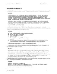
Consider the problem of satisfiability (SAT) [48, page 996]. We formally
define SAT in the next chapter, but for now consider the following problem.
Given the circuit depicted in Fig. 2.15, is there a set of values for the variables
(inputs) x and y that result in the circuit’s output z having the value 1?
X
Y
1 Read “big-oh of n”, or “oh of n”.
Fig. 2.15. Satisfiability circuit
Z