Image Reconstruction for 3D Lung Imaging - Department of Systems ...

More documents

Recommendations

Info

A.1 Introduction One of the most promising applications of Electrical Impedance Tomography (EIT) is for monitoring lung function [50] such as measuring the amount and distribution of inspired air. EIT images of the lung benefit from its large size and large conductivity contrast to other body tissues. Moreover there is a linear relationship between the measured tidal volume and the amplitude of EIT difference images (e.g. [94]). However, the constant of proportionality varies dramatically between subjects. Kunst et al [83] studied the variation in EIT image amplitude between subjects. Images of a given tidal volume 1 were compared between normals and groups with high parenchyma density (haemodialysis patients) and low parenchyma density (emphysema patients). Results were measured in terms of the sum of image pixels per litre of tidal volume. The emphysema group had significantly lower impedance change (11.6±6.4) than normals (18.6±4.2), while the haemodialysis group showed a significantly larger impedance change (30.5±13.1). Furthermore, during dialysis, the latter group showed impedance changes much closer to the normals (21.4 ± 8.6). These results show EIT in poor light: not only can measurements of the same tidal volume vary by a factor of three between patient groups, but even if calibration is performed, the calibration factor can undergo large changes rapidly. We are interested in understanding the cause of and compensating for this variability in image amplitude. In this paper we deal with the cause. Future work will look at compensation. In this paper, we propose that this effect is mainly caused by the assumption of homogeneity made in the formulation of difference images in EIT via the Jacobian matrix. In order to explore this effect, a finite element model of the thorax was constructed, and simulation data at different baseline lung conductivities generated. Subsequently, images were reconstructed from these data under different difference imaging assumptions, and compared to the results of Kunst et al [83]. A.2 Methods A.2.1 Image Reconstruction We consider EIT difference imaging, which is widely understood to improve reconstructed image stability in the presence of problems such as unknown contact impedance, inaccurate electrode positions, non linearity, and in the 2D case, the use of 2D approximations for 3D electrical fields [17][87]. We address the class of normalized one-step linearized reconstruction algorithms that calculate the normalized change in finite element conductivity distribution, x, due to a change in normalized difference signal, z, over a time interval (t1,t2). length(x) � Here x is defined as xi = (σ2,i − σ1,i) /σ1,i with σ1,i and σ2,i being the ith elements i of the vectors σ1 and σ2 respectively, and z is defined as zi = length(v) � i (v2,i − v1,i)/v1,i with v1,i and v2,i being the i th elements of the vectors v1 and v2 respectively. By convention we consider the signal at t1 to be the reference frame and the signal at t2 to be the data frame. For small changes around a background conductivity the relationship between x and z may be linearized as z = Hx + n (A.3) 1 Tidal Volume is the amount of air inhaled and exhaled during normal breathing, normally about between 500 and 1000ml. 119
where H is the Jacobian or sensitivity matrix calculated from a FEM (F(σ)), and n is the measurement system noise, assumed to be uncorrelated additive white Gaussian (AWGN). Each element i, j, of H is calculated as Hij = ∂zi � � and relates a small change in the � ∂xj σ0 i th difference measurement to a small change in the conductivity of j th element. H is a function of the FEM, the current injection pattern, and the background conductivity, σ0. Here σ0 is a vector containing the conductivity of each element of the mesh. In order to overcome the ill-conditioning of H we solve A.3 using the following regularized inverse ˆx = (H T WH + λ 2 R T R) −1 H T Wz = Bz (A.4) where ˆx is an estimate of the true change in conductivity distribution, R is a regularization matrix, λ is a scalar hyperparameter that controls the amount of regularization, and W models the system noise. The regularization matrix, R, is the spatially invariant Gaussian high pass filter of [4] with a cut-off frequency of 10% of the medium diameter. Hyperparameter selection was performed using the BestRes method [52]. Reconstruction algorithms for EIT difference images often assume that the background conductivity, σ0, of the region being imaged is homogeneous, and conductivity changes occur with respect to this baseline value. This assumption is clearly unwarranted for imaging of the thorax, where the lungs are significantly less conductive than other tissue. In order to modify the assumption of a homogeneous background conductivity, σ0 can be altered to account for the conductivity of the various tissues in the thorax. The sensitivity matrix, H, is then constructed from the modified σ0 and used to calculate the reconstructed image. 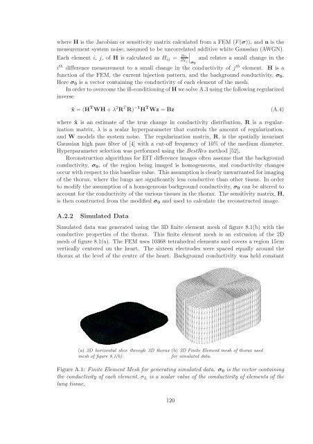A.2.2 Simulated Data Simulated data was generated using the 3D finite element mesh of figure 8.1(b) with the conductive properties of the thorax. This finite element mesh is an extrusion of the 2D mesh of figure 8.1(a). The FEM uses 10368 tetrahedral elements and covers a region 15cm vertically centered on the heart. The sixteen electrodes were spaced equally around the thorax at the level of the centre of the heart. Background conductivity was held constant (a) 2D horizontal slice through 3D thorax mesh of figure 8.1(b). (b) 3D Finite Element mesh of thorax used for simulated data. Figure A.1: Finite Element Mesh for generating simulated data. σ0 is the vector containing the conductivity of each element, σL is a scalar value of the conductivity of elements of the lung tissue. 120
Page 1 and 2:
Enhancements in Electrical Impedanc
Page 3 and 4:
Acknowledgements I would like to de
Page 5 and 6:
3.5 3D Considerations . . . . . . .
Page 7 and 8:
Bibliography 127 VITA 135 vii
Page 9 and 10:
4.8 GCV curves for different priors
Page 11 and 12:
7.15 Four layer tank used for 3D re
Page 13 and 14:
Discrete Variables • I is the mat
Page 15 and 16:
as opposed to anatomical imaging. W
Page 17 and 18:
to know how various alternative con
Page 19 and 20:
to noise however both algorithms pr
Page 21 and 22:
Chapter 2 Forward Problem 2.1 Descr
Page 23 and 24:
there are two primary types in EIT.
Page 25 and 26:
impedance, σ(�x,t) + jω(�x,t)
Page 27 and 28:
elying on a variational statement.
Page 29 and 30:
with Y11 = −Y12 − Y13, Y22 =
Page 31 and 32:
2.3.1.3 Derivation of Linear Interp
Page 33 and 34:
with Ci being the following column
Page 35 and 36:
Substitution of 2.24 into 2.21 yiel
Page 37 and 38:
where the superscript identifies th
Page 39 and 40:
2.3.3.4 Numerical Implementation of
Page 41 and 42:
is selected, measurements are taken
Page 43 and 44:
measurements of which only 104 are
Page 45 and 46:
Chapter 3 Reconstruction The proces
Page 47 and 48:
where the Jacobian is � H = T −
Page 49 and 50:
The condition number of a matrix is
Page 51 and 52:
2. As λ goes to zero, the un-regul
Page 53 and 54:
6. Evaluate a stopping rule. For ex
Page 55 and 56:
Finally Adler and Guardo define the
Page 57 and 58:
3.5 3D Considerations In EIT it is
Page 59 and 60:
Chapter 4 Objective Selection of Hy
Page 61 and 62:
initial conductivity x = ∆σ/σ0.
Page 63 and 64:
λ=0.0008 λ=0.0302 λ=0.0616 λ=6.
Page 65 and 66:
4.3.3 Generalized Cross-Validation
Page 67 and 68:
1. simulated data, generated using
Page 69 and 70:
GCV 1.8 1.6 1.4 1.2 1 0.8 0.6 0.4 0
Page 71 and 72:
a hyperparameter selection method,
Page 73 and 74:
1. Heuristic selections of hyperpar
Page 75 and 76:
human lung data. Keywords: regulari
Page 77 and 78:
fields when reconstructing in 2D [1
Page 79 and 80:
i and integrating across element j
Page 81 and 82: 5.2.5 Nodal Gaussian Filter The Gau
Page 83 and 84: Quantitative figures of merit are r
Page 85 and 86: (a) Rdiag BR=.236, SNR=.332 (b) Fil
Page 87 and 88: plane located halfway between the e
Page 89 and 90: models that are difficult or imposs
Page 91 and 92: 6.1 Introduction EIT attempts to ca
Page 93 and 94: 6.2.1 Image Reconstruction In order
Page 95 and 96: Aligned, fig 6.2(a) Planar Zigzag Z
Page 97 and 98: of reconstructions were calculated
Page 99 and 100: case normalized to the first and la
Page 101 and 102: Resolution (BR) Image Radial Positi
Page 103 and 104: configuration gave the worse overal
Page 105 and 106: Planar and Planar-offset configurat
Page 107 and 108: Chapter 7 Total Variation Regulariz
Page 109 and 110: on the conductivity vector, σ, whi
Page 111 and 112: a regularization penalty term a muc
Page 113 and 114: etween primal and dual optimal poin
Page 115 and 116: The optimization problem min x 1 2
Page 117 and 118: PD-IPM Algorithm ψ(σ) = 1 2 �F(
Page 119 and 120: (a) First step, TV solution. BRTV =
Page 121 and 122: Iteration 1 (a) Iteration 4 (d) Ite
Page 123 and 124: (a) L 2 solution with 2.5% AWGN, fi
Page 125 and 126: (a) i=1 (b) i=2 (c) i=3 (d) i=4 (e)
Page 127 and 128: Figure 7.15: Four layer tank used f
Page 129 and 130: can be solved with the algorithm. T
Page 131: Appendix: Variability in EIT Images
Page 135 and 136: (a) AσˆL = 33% (b) Aσ ˆL = 51%
Page 137 and 138: Figure A.4: Reconstructions with ho
Page 139 and 140: Figure A.7: Reconstructions with no
Page 141 and 142: [15] Barber DC, Brown BH, Applied p
Page 143 and 144: [49] Frerichs I, Hahn G, Hellige G,
Page 145 and 146: [83] Kunst PWA, Vonk Noordegraaf A,
Page 147 and 148: [116] Vauhkonen M, Lionheart WRB, H
show all

Image Reconstruction for 3D Lung Imaging - Department of Systems ...

You also want an ePaper? Increase the reach of your titles

Delete template?

Save as template?