Image Reconstruction for 3D Lung Imaging - Department of Systems ...

Kirchoff’s current law. The resulting potential field is calculated by solving the following
algebraic system of equations:
YV = I (2.8)
where Y is the global admittance matrix which is a function of the FEM and the conductivity,
V is a vector of nodal voltages
V = [u1,u2,...,uN] T
and I is the current vector which for the adjacent drive is a permutation of
I = [0,0,..., −1,1,...0] T
(2.9)
(2.10)
The non-zeros represent the current driven between a pair of electrodes while the zeros
represent the current at each node which is zero by Kirchoff’s current law. The two nonzero
elements of equation 2.10 are not necessarily adjacent elements of the vector I. By
convention ±1 are used as the current values, however when matching lab equipment one
uses the current values injected by the equipment, for example 5mA for the equipment in
our lab. Equation 2.8 is solved for the nodal voltages as V = Y−1I. Thus using the Direct
approach with the Gap model the forward problem can be viewed as using Kirchoff’s current
law to solve a large network assembled as a set of simultaneous linear equations.
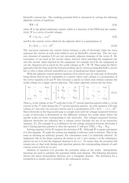
With the adjacent current pattern equation 2.8 is solved once for each pair of electrodes
being driven thus I can be assembled as a matrix where each column is a permutation of
the vector equation 2.10 and V then becomes a matrix in which each column contains the
nodal voltage for a single current injection. The entire algebraic system has the form:
⎡
⎤
u11 · · · · · · u1M
⎢
.
⎢ . ..
⎥
uij . ⎥
⎢
⎣
.
. uij
..
⎥
. ⎦ =
⎡
⎤−1
1 0 · · · 0
⎢ 0 Y22 · · · Y2N
⎥
⎢
⎣
.
. . ..
⎥
. ⎦
⎡
⎤
c11 · · · · · · c1M
⎢
.
⎢ . ..
⎥
cij . ⎥
⎢
⎣
.
. cij
..
⎥
. ⎦ (2.11)
u1M · · · · · · uNM
0 YN2 · · · YNN
c1M · · · · · · cNM
Thus uij is the voltage at the i th node due to the j th current injection pattern while cij is the
current at the i th node during the j th current injection pattern. As with equation 2.10 each
column of i has only two non-zero entries and is a permutation of I = [0,0,..., −1,1,...0] T .
Since electrodes in the Gap model map to a single node each the voltages measured between
a pair of electrodes is determined by the difference between two nodal values where the
specific nodes are those corresponding to the electrodes. The voltages measured between
adjacent electrodes are collected into a column vector through the use of an extraction
operator, T[]. For example if v9 is defined to be the voltage measured between electrodes 4
and 5 during injection pattern 2, then the operator T will give T[V]9 = V42 − V52.
Solving equation 2.8 for V requires the inversion of Y. Although Y is square and sparse
it is also singular. To make the system non-singular a reference node is selected. This is the
same as choosing an arbitrary ground. For convenience node 1 is arbitrarily selected. To
implement this in the linear equation all entries in row 1 and column 1 of the admittance
matrix are set to 0 and the diagonal elements is set to 1. To ensure that the potential will
remain zero at that node during each injection pattern the corresponding element of each
current vector in I is set to zero.
Solution of equation 2.11 provides the potential values at the nodes. Interpolation
functions are used to calculate the potential within each element. The following discussion
derives the linear interpolation function over a triangular element. The derivation for a
tetrahedron is similar and is included in the subsequent section.
17