Image Reconstruction for 3D Lung Imaging - Department of Systems ...

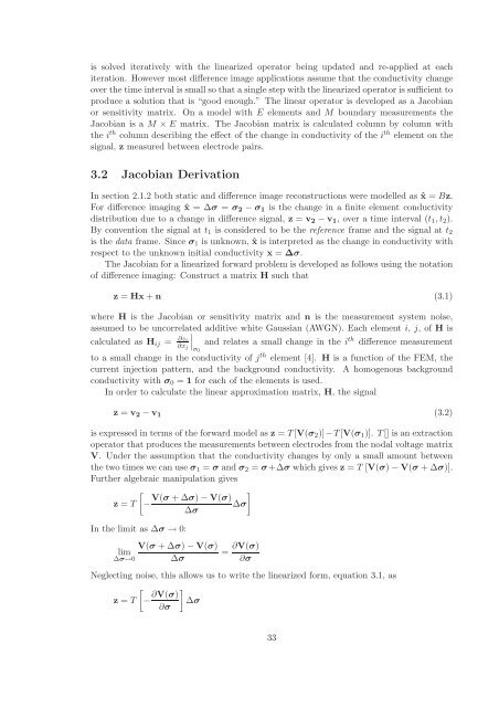
is solved iteratively with the linearized operator being updated and re-applied at each
iteration. However most difference image applications assume that the conductivity change
over the time interval is small so that a single step with the linearized operator is sufficient to
produce a solution that is “good enough.” The linear operator is developed as a Jacobian
or sensitivity matrix. On a model with E elements and M boundary measurements the
Jacobian is a M × E matrix. The Jacobian matrix is calculated column by column with
the i th column describing the effect of the change in conductivity of the i th element on the
signal, z measured between electrode pairs.
3.2 Jacobian Derivation
In section 2.1.2 both static and difference image reconstructions were modelled as ˆx = Bz.
For difference imaging ˆx = ∆σ = σ2 − σ1 is the change in a finite element conductivity
distribution due to a change in difference signal, z = v2 − v1, over a time interval (t1,t2).
By convention the signal at t1 is considered to be the reference frame and the signal at t2
is the data frame. Since σ1 is unknown, ˆx is interpreted as the change in conductivity with
respect to the unknown initial conductivity x = ∆σ.
The Jacobian for a linearized forward problem is developed as follows using the notation
of difference imaging: Construct a matrix H such that
z = Hx + n (3.1)
where H is the Jacobian or sensitivity matrix and n is the measurement system noise,
assumed to be uncorrelated additive white Gaussian (AWGN). Each element i, j, of H is
calculated as Hij = ∂zi
�
�
and relates a small change in the ith difference measurement
� ∂xj σ0
to a small change in the conductivity of jth element [4]. H is a function of the FEM, the
current injection pattern, and the background conductivity. A homogenous background
conductivity with σ0 = 1 for each of the elements is used.
In order to calculate the linear approximation matrix, H, the signal
z = v2 − v1
(3.2)
is expressed in terms of the forward model as z = T[V(σ2)]−T[V(σ1)]. T[] is an extraction
operator that produces the measurements between electrodes from the nodal voltage matrix
V. Under the assumption that the conductivity changes by only a small amount between
the two times we can use σ1 = σ and σ2 = σ+∆σ which gives z = T [V(σ) − V(σ + ∆σ)].
Further algebraic manipulation gives
�
�
V(σ + ∆σ) − V(σ)
z = T − ∆σ
∆σ
In the limit as ∆σ → 0:
V(σ + ∆σ) − V(σ)
lim
∆σ→0 ∆σ
= ∂V(σ)
∂σ
Neglecting noise, this allows us to write the linearized form, equation 3.1, as
�
z = T − ∂V(σ)
�
∆σ
∂σ
33