Image Reconstruction for 3D Lung Imaging - Department of Systems ...

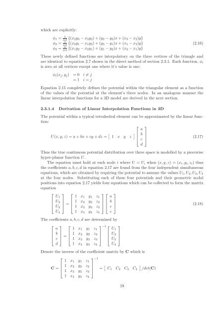
which are explicitly:
φ1 = 1
2A {(x2y3 − x3y2) + (y2 − y3)x + (x3 − x2)y}
φ2 = 1
2A {(x3y1 − x1y3) + (y3 − y1)x + (x1 − x3)y}
φ3 = 1
2A {(x1y2 − x2y1) + (y1 − y2)x + (x2 − x1)y}
(2.16)
These newly defined functions are interpolatory on the three vertices of the triangle and
are identical to equation 2.7 shown in the direct method of section 2.3.1. Each function, φi
is zero at all vertices except one where it’s value is one:
φi(xj,yj) = 0 i �= j
= 1 i = j
Equation 2.15 completely defines the potential within the triangular element as a function
of the values of the potential at the element’s three nodes. In an analogous manner the
linear interpolation functions for a 3D model are derived in the next section.
2.3.1.4 Derivation of Linear Interpolation Functions in 3D
The potential within a typical tetrahedral element can be approximated by the linear function:
U(x,y,z) = a + bx + cy + dz = � 1 x y z �
⎡ ⎤
a
⎢ b ⎥
⎣ c ⎦
(2.17)
d
Thus the true continuous potential distribution over three space is modelled by a piecewise
hyper-planar function U.
The equation must hold at each node i where U = Ui when (x,y,z) = (xi,yi,zi) thus
the coefficients a,b,c,d in equation 2.17 are found from the four independent simultaneous
equations, which are obtained by requiring the potential to assume the values U1,U2,U3,U4
at the four nodes. Substituting each of these four potentials and their geometric nodal
positions into equation 2.17 yields four equations which can be collected to form the matrix
equation
⎡
⎢
⎣
U1
U2
U3
U4
⎤
⎥
⎦ =
⎡
⎢
⎣
1 x1 y1 z1
1 x2 y2 z2
1 x3 y3 z3
1 x4 y4 z4
⎤ ⎡
⎥ ⎢
⎥ ⎢
⎦ ⎣
a
b
c
c
⎤
⎥
⎦
The coefficients a,b,c,d are determined by
⎡ ⎤
a
⎢ b ⎥
⎣ c ⎦
d
=
⎡
⎤−1
⎡ ⎤
U1
⎢
⎥ ⎢ U2 ⎥
⎢
⎥ ⎢ ⎥
⎣
⎦ ⎣ U3 ⎦
1 x1 y1 z1
1 x2 y2 z2
1 x3 y3 z3
1 x4 y4 z4
Denote the inverse of the coefficient matrix by C which is
⎡
⎤
C =
⎢
⎣
1 x1 y1 z1
1 x2 y2 z2
1 x3 y3 z3
1 x4 y4 z4
⎥
⎦
−1
U4
= � C1 C2 C3 C4
19
� /det(C)
(2.18)