New Statistical Algorithms for the Analysis of Mass - FU Berlin, FB MI ...

34 CHAPTER 3. MATHEMATICAL MODELING AND ALGORITHMS
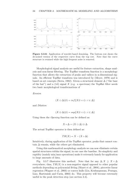
Figure 3.3.6: Application of wavelet-based denoising. The buttom row shows the
de-noised version of the respective curve from the top row. Note that the curve
structure is retained while the high frequent noise is removed.
Morphological signal analysis are useful for feature extraction, shape analysis
and non-linear filtering. The TopHat transform function is a morphology
function that allows the extraction of peaks and valleys in n-dimensional signals.
An efficient TopHat transform was introduced by (Meyer, 1979) and is
based on set concepts (Serra, 1982). Given a structural element ∆ (“the base
of the hat”) and a (1d) signal X (e.g. a spectrum) the TopHat filter needs
two basic morphological transformations of
Erosion
and Dilation
(X ⊖ ∆)(t) = inf{X(t + i) : i ∈ ∆}
(X ⊕ ∆)(t) = sup{X(t + i) : i ∈ ∆}
Using these the Opening function can be defined as:
X ◦ ∆ = (X ⊖ ∆) ⊕ ∆
The actual TopHat operator is then defined as:
T H(X) = X − (X ◦ ∆)
Intuitively, during application of the TopHat operator, peaks that cannot contain
∆ remain, while the others get eliminated.
Using this mathematical morphology analysis we can now eliminate certain
spatial structures within the signal, in our case the baseline. Its simplicity and
rapidity (mainly min/max operations) make it extremely handy for application
to large amounts of data.
Fig. 3.3.7 illustrates this method. Note that for any ∆, X ≥ X ◦ ∆
everywhere; thus, T H(X) is a non-negative signal opposed to other popular
methods depending on polynomial fitting (Mazet et al., 2004), piecewise linear
regression (Wagner et al., 2003) or convex hulls (Liu, Krishnapuram, Pratapa,
Liao, Hartemink and Carin, 2003) do. This property will become extremely
useful in the peak detection step (see section 3.4).