Diploma thesis

Applied to Eq. 3.2 (I1 = I2 = I ′ p(ω)), this requires an integration over the pump
spectrum, to consider all different mixing possibilities for one particular output
SFG frequency. For the sake of a clear arrangement, we merged all slowly varying
variables into the factors K and K’:
� ∞ � ∞
I3(ω3) = dω1
0
� ∞
=
0
0
dω2K ′ I 2 pe − (ω 1 −ωp)2
2σ 2 p e − (ω 2 −ωp)2
2σ 2 p sinc 2
dω1KI 2 pe − (ω 1 −ωp)2
2σ 2 p e − (ω 1 −ω 3 −ωp)2
2σ 2 p sinc 2
� �
∆kL
2
� �
∆kL
2
(3.7)
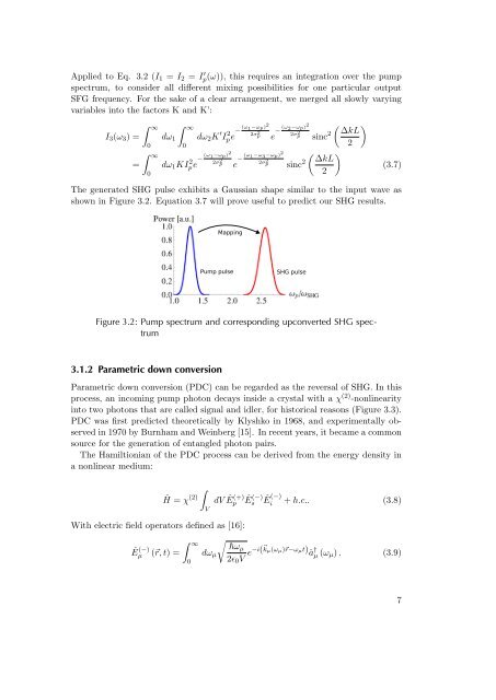
The generated SHG pulse exhibits a Gaussian shape similar to the input wave as
shown in Figure 3.2. Equation 3.7 will prove useful to predict our SHG results.
Figure 3.2: Pump spectrum and corresponding upconverted SHG spectrum
3.1.2 Parametric down conversion
Parametric down conversion (PDC) can be regarded as the reversal of SHG. In this
process, an incoming pump photon decays inside a crystal with a χ (2) -nonlinearity
into two photons that are called signal and idler, for historical reasons (Figure 3.3).
PDC was first predicted theoretically by Klyshko in 1968, and experimentally observed
in 1970 by Burnham and Weinberg [15]. In recent years, it became a common
source for the generation of entangled photon pairs.
The Hamiltionian of the PDC process can be derived from the energy density in
a nonlinear medium:
ˆH = χ (2)
�
V
dV Ê(+)
p
With electric field operators defined as [16]:
Ê (−)
s Ê (−)
i + h.c.. (3.8)
Ê (−)
� �
∞ �ωµ
µ (�r, t) = dωµ
0 2ɛ0V e−i(� kµ(ωµ)�r−ωµt) †
â µ (ωµ) . (3.9)
7