Diploma thesis

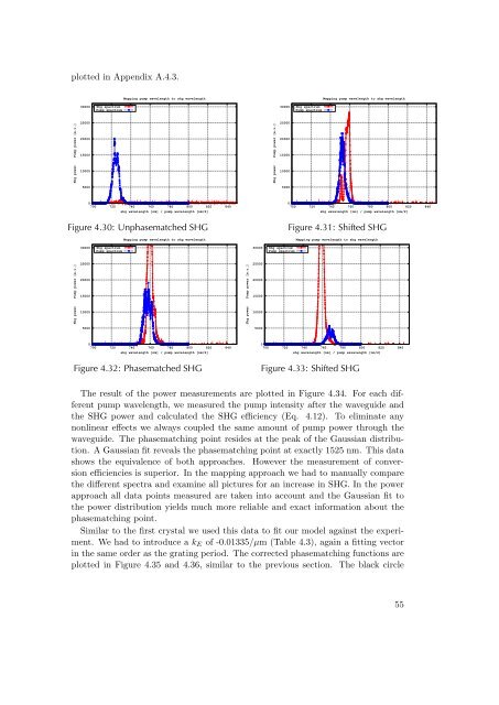
plotted in Appendix A.4.3.
Shg power Pump power [a.u.]
30000
25000
20000
15000
10000
5000
Shg spectrum
Pump spectrum
Mapping pump wavelength to shg wavelength
0
700 720 740 760 780 800 820 840
shg wavelength [nm] / pump wavelength [nm/2]
Figure 4.30: Unphasematched SHG
Shg power Pump power [a.u.]
30000
25000
20000
15000
10000
5000
Shg spectrum
Pump spectrum
Mapping pump wavelength to shg wavelength
0
700 720 740 760 780 800 820 840
shg wavelength [nm] / pump wavelength [nm/2]
Figure 4.32: Phasematched SHG
Shg power Pump power [a.u.]
30000
25000
20000
15000
10000
5000
Shg power Pump power [a.u.]
30000
25000
20000
15000
10000
5000
Shg spectrum
Pump spectrum
Shg spectrum
Pump spectrum
Mapping pump wavelength to shg wavelength
0
700 720 740 760 780 800 820 840
shg wavelength [nm] / pump wavelength [nm/2]
Figure 4.31: Shifted SHG
Mapping pump wavelength to shg wavelength
0
700 720 740 760 780 800 820 840
shg wavelength [nm] / pump wavelength [nm/2]
Figure 4.33: Shifted SHG
The result of the power measurements are plotted in Figure 4.34. For each different
pump wavelength, we measured the pump intensity after the waveguide and
the SHG power and calculated the SHG efficiency (Eq. 4.12). To eliminate any
nonlinear effects we always coupled the same amount of pump power through the
waveguide. The phasematching point resides at the peak of the Gaussian distribution.
A Gaussian fit reveals the phasematching point at exactly 1525 nm. This data
shows the equivalence of both approaches. However the measurement of conversion
efficiencies is superior. In the mapping approach we had to manually compare
the different spectra and examine all pictures for an increase in SHG. In the power
approach all data points measured are taken into account and the Gaussian fit to
the power distribution yields much more reliable and exact information about the
phasematching point.
Similar to the first crystal we used this data to fit our model against the experiment.
We had to introduce a kE of -0.01335/µm (Table 4.3), again a fitting vector
in the same order as the grating period. The corrected phasematching functions are
plotted in Figure 4.35 and 4.36, similar to the previous section. The black circle
55