Diploma thesis

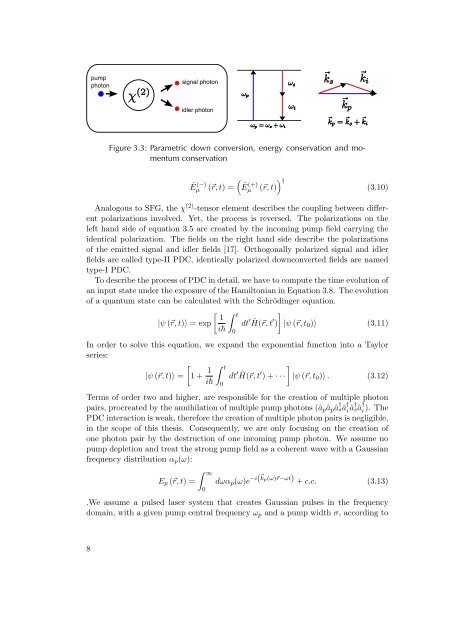
Figure 3.3: Parametric down conversion, energy conservation and momentum
conservation
Ê (−)
� � †
(+)
µ (�r, t) = Ê µ (�r, t)
(3.10)
Analogous to SFG, the χ (2) -tensor element describes the coupling between different
polarizations involved. Yet, the process is reversed. The polarizations on the
left hand side of equation 3.5 are created by the incoming pump field carrying the
identical polarization. The fields on the right hand side describe the polarizations
of the emitted signal and idler fields [17]. Orthogonally polarized signal and idler
fields are called type-II PDC, identically polarized downconverted fields are named
type-I PDC.
To describe the process of PDC in detail, we have to compute the time evolution of
an input state under the exposure of the Hamiltonian in Equation 3.8. The evolution
of a quantum state can be calculated with the Schrödinger equation.
� � t 1
|ψ (�r, t)〉 = exp dt
i�
′ �
H(�r, ˆ ′
t ) |ψ (�r, t0)〉 (3.11)
0
In order to solve this equation, we expand the exponential function into a Taylor
series:
|ψ (�r, t)〉 =
�
1 + 1
� t
dt
i� 0
′ �
H(�r, ˆ ′
t ) + · · · |ψ (�r, t0)〉 . (3.12)
Terms of order two and higher, are responsible for the creation of multiple photon
pairs, procreated by the annihilation of multiple pump photons (âpâpâ † sâ †
i ↠s⠆
i ). The
PDC interaction is weak, therefore the creation of multiple photon pairs is negligible,
in the scope of this thesis. Consequently, we are only focusing on the creation of
one photon pair by the destruction of one incoming pump photon. We assume no
pump depletion and treat the strong pump field as a coherent wave with a Gaussian
frequency distribution αp(ω):
� ∞
Ep (�r, t) =
0
dωαp(ω)e −i(� kp(ω)�r−ωt) + c.c. (3.13)
.We assume a pulsed laser system that creates Gaussian pulses in the frequency
domain, with a given pump central frequency ωp and a pump width σ, according to
8