Djeraba Aicha - Université des Sciences et de la Technologie d ...
Djeraba Aicha - Université des Sciences et de la Technologie d ...
Djeraba Aicha - Université des Sciences et de la Technologie d ...

You also want an ePaper? Increase the reach of your titles
YUMPU automatically turns print PDFs into web optimized ePapers that Google loves.
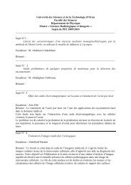
Figure I.5 : L’idée <strong>de</strong> Thouless. Il<br />
construit un échantillon <strong>de</strong> taille<br />
macroscopique à partir d’un<br />
échantillon microscopique en<br />
doub<strong>la</strong>nt <strong>la</strong> taille <strong>de</strong> celui-ci <strong>de</strong><br />
manière itérative. Par exemple, il<br />
passe d’un échantillon cubique<br />
<strong>de</strong> taille (L) d en dimension d à un<br />
échantillon <strong>de</strong> taille (2L) d puis<br />
(4L) d ………….<br />
Thouless a montré que g (Lb)<br />
s’exprime uniquement en fonction <strong>de</strong> g (L)<br />
<strong>et</strong> <strong>de</strong>b .<br />
A partir <strong>de</strong> c<strong>et</strong>te démonstration Abrahams <strong>et</strong> al [3] ont montré que lorsqu’on<br />
augmente <strong>la</strong> taille du système en combinant <strong><strong>de</strong>s</strong> blocs <strong>de</strong> taille donnée, <strong>la</strong><br />
conductivité varie <strong>de</strong> manière à ce que :<br />
d ln( g(<br />
L)<br />
d ln( L)<br />
= β ( g(<br />
L))<br />
(I.11)<br />
La fonction β ainsi construite ne dépend que <strong>de</strong> g .<br />
Il est possible <strong>de</strong> déterminer les limites asymptotiques <strong>de</strong> <strong>la</strong> fonction β (g)<br />
, à<br />
gran<strong><strong>de</strong>s</strong> <strong>et</strong> à p<strong>et</strong>ites valeurs <strong>de</strong> g , par <strong><strong>de</strong>s</strong> arguments généraux <strong>de</strong> <strong>la</strong> physique.<br />
Pour g grand <strong>la</strong> théorie macroscopique du transport est applicable, conduisant<br />
à :<br />
d −2<br />
G(<br />
L)<br />
= σ L <strong>et</strong> lim β ( g)<br />
= d − 2<br />
(I.12)<br />
g→∞<br />
Dans c<strong>et</strong>te même limite, on peut aller plus loin en utilisant <strong>la</strong> théorie <strong>de</strong> <strong>la</strong><br />
localisation faible qui donne un développement en W V = 1 g :<br />
β ( g)<br />
= d − 2 − a g + ο(1<br />
g)<br />
(I.13)<br />
Pour g p<strong>et</strong>it, on tombe dans le régime localisé, <strong>et</strong> on a :<br />
−L<br />
λ<br />
G = g<br />
0e<br />
<strong>et</strong> lim β (g) = ln(g g<br />
0<br />
( d))<br />
g→0<br />
(I.14)<br />
- 15 -