THÈS EE - CESBIO - Université Toulouse III - Paul Sabatier

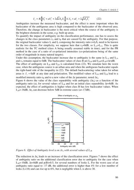
Chapitre 3. Article 12 2IaK S0 + aSs+ 2 aS0Ss≤ I0+ aIs+ 2 aI0= I (22)Ambiguities increase the measured backscatter, and the effect is more important when thebackscatter of the ambiguous area is high compared to the backscatter of the observed area.Therefore, the change in backscatter is the most critical when the source of the ambiguity isthe brightest elements in the scene, e.g. built up areas.To quantify the impact of ambiguity on the classification performance, one has to assess thechanges in the class parameters r A and r B that are caused by the ambiguity. For that purpose,the original backscatter values I 1 and I 2 composing the intensity ratio r=I 2 /I 1 need to be knownfor the two classes. For simplicity, we suppose here that r A =0dB, so I 1,A =I 2,A . This is quiterealistic for the TC method (class A being usually assumed stable in time), and for the PRmethod in the case of a ratio of co-polarized intensities (co-polarizations being of the sameorder of magnitude in many natural targets).Under this assumption, the backscatter increase due to ambiguity is the same in I 1,A and I 2,Aand r A remains equal to 0dB. The backscatter values of class B are I 1,B and I 2,B =(I 1,B +∆r)dB.The effect of ambiguity on I 1,B and I 2,B is calculated from (22). We simulate here the worstcase, when the ambiguous source is an urban area and when the ambiguous backscatter equalsthe right-hand side of the inequality in (22). The default backscattering value taken for urbanareas is I s= 0dBat any date and polarization. The modified values of I 1,B and I 2,B lead to amodified intensity ratio r B and to a new value of the ∆r parameter, noted ∆r a .Figure 6 shows the value of the class separability with ambiguity (∆r a ) as a function of theambiguity ratio (a), for several values of I 1,B and for an initial class separability ∆r=8dB. Asexpected, the effect of ambiguities is higher when class B has low backscatter values. WhenI 1,B =-16dB, ∆r a can decrease below 5dB in extreme cases (a=-17dB).sEffect of ambiguity on ∆r a876∆r a(dB)54I 1,B=-16dB3-14dB-12dB2 -10dB-8dB1 -6dB-4dB0-40 -35 -30 -25 -20 -15Ambiguity ratio (dB)Figure 6. Effect of Ambiguity level a on ∆r a with several values of I 1,B .The reduction in ∆r a leads to an increase of the classification error. Figures 7 shows the effectof ambiguity ratio on the additional classification error due to ambiguity for the case whenI 1,B =-10dB, ∆r=8dB and p(B)=0.5, for several numbers of looks L. For the worst case of anambiguity ratio equal to -17 dB, the additional error is higher than 4% for a low number oflooks (L