THÃS EE - CESBIO - UniversitÃ© Toulouse III - Paul Sabatier

More documents

Recommendations

Info

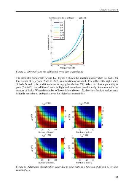
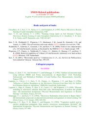
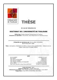
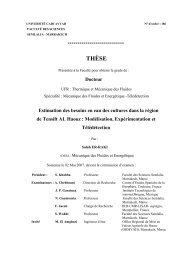
Chapitre 3. Article 1Additional error (%)Additional error due to ambiguity - p(B)=0.58L=17 L=2L=46 L=8L=165L=32L=6443210-40 -35 -30 -25 -20 -15Ambiguity ratio (dB)Figure 7. Effect of A on the additional error due to ambiguityThe error also varies with ∆r and I 1,B . Figure 8 shows the additional error when a=-17dB, forfour values of I 1,B from -20dB to -5dB, as a function of ∆r and L. For sufficiently high valuesof both ∆r and L, the additional error is negligible (below 2%). When the class separability ispoor (∆r
Chapitre 3. Article 1In summary, ambiguities can have a critical impact on the performance of the classificationmethods when the ambiguity ratio is high (a=-17dB), if the class separability is low and/or ifthe number of looks is low. For a given SAR system, the methods should therefore be appliedonly when the classes are highly separable. Further simulations show that when the ambiguityis better than -30dB, the additional error is however limited to 6% in the very worst case,including poorly separable classes.B. Impact of the temporal samplingIn both methods, it is generally implicitly supposed that the class separability, measured by∆r, is due mostly to the outstanding behaviour of the intensity ratio (TC or PR) of one class ofinterest, which reaches peculiar values in time, while the intensity ratio of the other classremains relatively constant around its typical value. We suppose here that the class of interestis class B, and that its intensity ratio is remarkable because of its high values (r B >r A ).In some applications, the outstanding radiometric behaviour of class B is caused by a pointevent, and lasts forever after the event. In that case, the timing of the data acquisitions is notvery important, provided one date is available after the event for the PR method, and one datebefore and one after for the TC method. Events such as deforestation or urbanization wouldbe illustrative of this category.In other situations, the outstanding behaviour of class B is caused by a phenomenon, whichlasts for a finite period during which the intensity ratio of class B expresses its particularity,and then stops. Applications such as crop monitoring or flood monitoring, are concerned bythis approach. The ∆r parameter then represents the theoretical optimal class separabilityobtained when data are acquired at the optimal dates. In the multitemporal case introduced inII.D., the value of the observed class separability will depend on the timing of the availableacquisitions, and on the temporal backscattering profiles of the two classes during the periodwhen the phenomenon occurs. The temporal sampling of the acquisitions is an importantparameter in this case, as a high observation frequency will increase the probability to haveoptimal dates in the available dataset.In this sub-section, temporal backscattering profiles are modelled to simulate the typicalbehaviour of the two classes likely to be involved in classification schemes based on thetemporal change or the polarization ratio. These modelled profiles are then used to assess theeffect of the observation frequency on the classification performance.1) Theoretical data modelWe model here the backscattering profiles of the two classes during the period when thephenomenon occurs, which is assumed to last for c days.a) Temporal change methodWe illustrate the case corresponding for class B to a temporal backscattering increase, i.e. apositive intensity ratio. Therefore the multitemporal classification feature is⎡ Ip,dj⎤rTC, multi= max ⎢ ⎥ , where p is the polarization and (di) i=1:N represent the dates in thei,j>i⎢⎣Ip,di ⎥⎦available time-series, as suggested in II.D.1.88
Page 4 and 5:
AbstractBecause of the importance o
Page 6 and 7:
que Monique, Delphine et Maud à l
Page 8 and 9:
Enfin, dans le cadre d’un troisi
Page 12 and 13:
6.2. Perspectives..................
Page 14 and 15:
Liste des tableauxTableau 1. Liste
Page 16 and 17:
Chapitre 1. Introduction générale
Page 18 and 19:
Page 20 and 21:
Page 22 and 23:
Page 24 and 25:
Page 26 and 27:
Page 28 and 29:
Page 30 and 31:
Page 32 and 33:
Page 34 and 35:
Page 36 and 37:
Page 38 and 39: Chapitre 1. Introduction générale
Page 40 and 41: Chapitre 1. Introduction générale
Page 42 and 43: Chapitre 2. Principes de l’imager
Page 62 and 63: Chapitre 3. Modèle d’erreur pour
Page 74 and 75: Chapitre 3. Article 12011, Sentinel
Page 76 and 77: Chapitre 3. Article 1rrB⎛ p(A)⎞
Page 78 and 79: Chapitre 3. Article 1- p(B), the a
Page 80 and 81: Chapitre 3. Article 1imperfections,
Page 82 and 83: Chapitre 3. Article 11.210.80.60.40
Page 84 and 85: Chapitre 3. Article 1and p(B)=0.5 (
Page 86 and 87: Chapitre 3. Article 122∆ 2δShv+
Page 90 and 91: Chapitre 3. Article 1As suggested i
Page 92 and 93: Chapitre 3. Article 1Particular val
Page 94 and 95: Chapitre 3. Article 1Table 1 summar
Page 96 and 97: Chapitre 3. Article 1The methods ar
Page 98 and 99: Chapitre 3. Article 1As predicted b
Page 100 and 101: Chapitre 3. Article 1Considering th
Page 102 and 103: Chapitre 4. Cartographie des riziè
Page 110 and 111: Chapitre 4. Article 2109
Page 124 and 125: Chapitre 5. Article 3USE OF ENVISAT
Page 126 and 127: Chapitre 5. Article 3during the rep
Page 128 and 129: Chapitre 5. Article 3which is plant
Page 130 and 131: Chapitre 5. Article 3the whole prov
Page 132 and 133: Chapitre 5. Article 3The 36 VGT-S10
Page 134 and 135: Chapitre 5. Article 3tTCTCTCTCr⎛
Page 136 and 137: Chapitre 5. Article 3Figure 7. Rice
Page 138 and 139:
Chapitre 5. Article 3Table 3. Plant
Page 140 and 141:
Chapitre 5. Article 3Table 5. Retri
Page 142 and 143:
Chapitre 5. Article 3Tien GiangMTC
Page 144 and 145:
Chapitre 5. Article 3Le Toan, T., R
Page 146 and 147:
Chapitre 6. Conclusion généraleLa
Page 148 and 149:
Chapitre 6. Conclusion généraleco
Page 150 and 151:
Annexe A. Rapport final du projet
Page 152 and 153:
Page 154 and 155:
Page 156 and 157:
Annexe B. Présentation du projet
Page 158 and 159:
Annexe B. Présentation du projet
Page 160 and 161:
Annexe C. Article 4Annexe C159
Page 162 and 163:
Annexe C. Article 4161
Page 164 and 165:
Page 166 and 167:
Page 168 and 169:
Page 170 and 171:
Page 172 and 173:
Page 174 and 175:
Page 176 and 177:
Annexe D. Article 5Annexe D175
Page 178 and 179:
Annexe D. Article 5177
Page 180 and 181:
Page 182 and 183:
Page 184 and 185:
Bibliographie[1] United Nations Dep
Page 186 and 187:
[29] Lee J.-S., Grunes M.R., Pottie
show all

THÃS EE - CESBIO - UniversitÃ© Toulouse III - Paul Sabatier

Create successful ePaper yourself

Delete template?

Save as template?

THÃS EE - CESBIO - UniversitÃ© Toulouse III - Paul Sabatier