Capitolo_11-Generatori_di_segnali_sinusoidali
Capitolo_11-Generatori_di_segnali_sinusoidali
Capitolo_11-Generatori_di_segnali_sinusoidali

Create successful ePaper yourself
Turn your PDF publications into a flip-book with our unique Google optimized e-Paper software.
50 <strong>Capitolo</strong> <strong>11</strong><br />
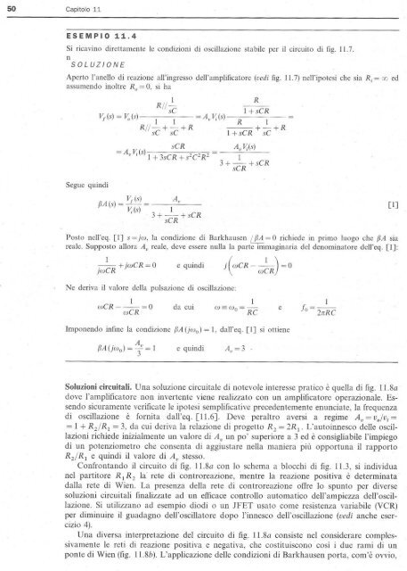
ESEMPIO <strong>11</strong>.4<br />
Si ricavino <strong>di</strong>rettamente le con<strong>di</strong>zioni <strong>di</strong> oscillazione stabile per il circuito <strong>di</strong> fig. <strong>11</strong>.7.<br />
n<br />
SOLUZIONE<br />
Aperto l'anello <strong>di</strong> reazione all'ingresso dell'amplificatore (ve<strong>di</strong> fig. <strong>11</strong>.7) nell'ipotesi che sia Rj = 00 ed<br />
assumendo inoltre Ro = O, si ha<br />
l R<br />
R//- -<br />
sC 1+ sCR<br />
Vf (s) = Va (s) l 1 = Av V; (s) R 1<br />
R//-+-+R +-+R<br />
sC sC l +sCR sC<br />
= AvV;(s) 1 + 3sCR +S2C 2 R 2<br />
Segue quin<strong>di</strong> A<br />
V/(s) = v<br />
f3A (s) = V (s) 3 + _1_. + sCR<br />
' sCR<br />
sCR _ Av V;(s)<br />
- 3+ S~R +sCR<br />
Posto nell'eq. [IJ s =jw, la con<strong>di</strong>zione <strong>di</strong> Barkhausen / [JA = O richiede in primo luogo che [JA sia<br />
reale. Supposto allora Av reale, deve essere nulla la parte immaginaria del denominatore dell'eq. [1]:<br />
1<br />
jwCR +jwCR = O c quin<strong>di</strong><br />
Ne deriva il valore della pulsazione <strong>di</strong> oscillazione:<br />
l =0<br />
wCR- wCR da cui<br />
1<br />
w=wo= RC e<br />
Imponendo infine la con<strong>di</strong>zione [JA (jw o ) = 1, dall'eq. [lJ si ottiene<br />
e quin<strong>di</strong><br />
1<br />
j~ = 2nRC<br />
Soluzioni circuitali. Una soluzione circuitale <strong>di</strong> notevole interesse pratico è quella <strong>di</strong> fig. <strong>11</strong>.8a<br />
dove l'amplificatore non invertente viene realizzato con un amplificatore operazionale. Essendo<br />
sicuramente verificate le ipotesi semplificati ve precedentemente enunciate, la frequenza<br />
<strong>di</strong> oscillazione è fornita dall'eq. [<strong>11</strong>.6]. Deve peraltro aversi a regime Av = vJu j =<br />
= 1+ R2/R1 = 3, da cui deriva la relazione <strong>di</strong> progetto R 2 = 2R 1 . L'autoinnesco delle oscillazioni<br />
richiede inizialmente un valore <strong>di</strong> Av un po' superiore a 3 ed è consigliabile l'impiego<br />
<strong>di</strong> un potenziometro che consenta <strong>di</strong> aggiustare nella maniera più opportuna il rapporto<br />
R2/ R 1 e quin<strong>di</strong> il valore <strong>di</strong> Av stesso.<br />
Confrontando il circuito <strong>di</strong> fig. Il.8a con lo schema a blocchi <strong>di</strong> fig. <strong>11</strong>.3, si in<strong>di</strong>vidua<br />
nel partitore R 1 R 2 la' rete <strong>di</strong> controreazione, mentre la reazione positiva è determinata<br />
dalla rete <strong>di</strong> Wien. La presenza della rete <strong>di</strong> controreazione offre lo spunto per <strong>di</strong>verse<br />
soluzioni circuitali finalizzate ad un efficace controllo automatico dell'ampiezza dell'oscillazione.<br />
Si utilizzano ad esempio <strong>di</strong>o<strong>di</strong> o un JFET usato come resistenza variabile (VCR)<br />
per <strong>di</strong>minuire il guadagno dell'oscillatore dopo l'innesco dell'oscillazione (ve<strong>di</strong> anche esercizio<br />
4).<br />
Una <strong>di</strong>versa interpretazione del circuito <strong>di</strong> fig. 1l.8a consiste nel considerare complessivamente<br />
le reti <strong>di</strong> reazione positiva e negativa, che costituiscono cosÌ i due rami <strong>di</strong> un<br />
ponte <strong>di</strong> Wien (fig. <strong>11</strong>.86). L'applicazione delle con<strong>di</strong>zioni <strong>di</strong> Barkhausen porta, com'è ovvio,<br />
[IJ