Dispensa di modelli lineari in R - Dipartimento di Statistica

CAPITOLO 3. DISTRIBUZIONI E STUDI DI SIMULAZIONE 33
Density
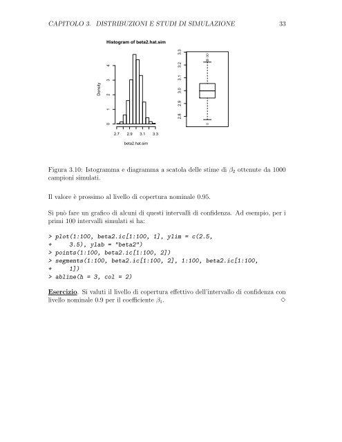
Histogram of beta2.hat.sim
0 1 2 3 4
2.7 2.9 3.1 3.3
beta2.hat.sim
Figura 3.10: Istogramma e diagramma a scatola delle stime di β2 ottenute da 1000
campioni simulati.
Il valore è prossimo al livello di copertura nominale 0.95.
Si può fare un grafico di alcuni di questi intervalli di confidenza. Ad esempio, per i
primi 100 intervalli simulati si ha:
> plot(1:100, beta2.ic[1:100, 1], ylim = c(2.5,
+ 3.5), ylab = "beta2")
> points(1:100, beta2.ic[1:100, 2])
> segments(1:100, beta2.ic[1:100, 2], 1:100, beta2.ic[1:100,
+ 1])
> abline(h = 3, col = 2)
Esercizio. Si valuti il livello di copertura effettivo dell’intervallo di confidenza con
livello nominale 0.9 per il coefficiente β1. ✸
2.8 2.9 3.0 3.1 3.2 3.3
●
●
●