Dispensa di modelli lineari in R - Dipartimento di Statistica

CAPITOLO 6. TEST T DI STUDENT 54
Frequency
Sample Quantiles
0 2 4 6 8
15 25 35 45
Histogram of RS
10 20 30 40
●
RS
Normal Q−Q Plot
● ●
●
●
●●
●
●
●●●
●
● ●
●
●
●●
● ●
●
−2 −1 0 1 2
Theoretical Quantiles
●
Frequency
Sample Quantiles
0 2 4 6
10 30 50
Histogram of SS
10 20 30 40 50
●
SS
Normal Q−Q Plot
●
●
●
●
●
●
●
●
● ●
●
●
●
●
●
● ●
●
−2 −1 0 1 2
Theoretical Quantiles
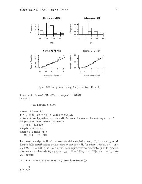
Figura 6.2: Istogrammi e qq-plot per le linee RS e SS.
> test test
Two Sample t-test
data: RS and SS
t = 0.6521, df = 48, p-value = 0.5175
alternative hypothesis: true difference in means is not equal to 0
95 percent confidence interval:
-3.3919 6.6479
sample estimates:
mean of x mean of y
25.256 23.628
La quantità t riporta il valore osservato della statistica test, t oss ; df sono i gradi di
libertà della distribuzione della statistica test sotto H0 (in questo caso n1 + n2 − 2 =
25 + 25 − 2 = 48); p-value è il livello di significatività osservato quando l’ipotesi
alternativa è bilaterale H1 : µRS = µSS, α oss = 2 PrH0(t > |t oss |), con t ∼ t48 sotto
H0. Infatti:
> 2 * (1 - pt(test$statistic, test$parameter))
t
0.51747
●