Dispensa di modelli lineari in R - Dipartimento di Statistica

CAPITOLO 5. COSTRUZIONE DEL MODELLO E ANALISI DEI RESIDUI 48
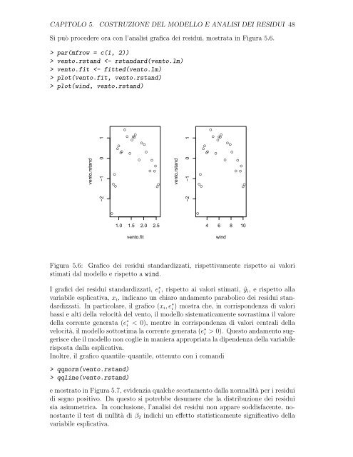
Si può procedere ora con l’analisi grafica dei residui, mostrata in Figura 5.6.
> par(mfrow = c(1, 2))
> vento.rstand vento.fit plot(vento.fit, vento.rstand)
> plot(wind, vento.rstand)
vento.rstand
−2 −1 0 1
●
●
●
●
●
●
●
●
●
● ●
●
●
●
●
●
●
●
●
● ●
●
●
1.0 1.5 2.0 2.5
vento.fit
−2 −1 0 1
●
●
●
●
●
●
●
●
●
● ●
●
●
●
●
●
●
●
●
● ●
●
●
4 6 8 10
Figura 5.6: Grafico dei residui standardizzati, rispettivamente rispetto ai valori
stimati dal modello e rispetto a wind.
vento.rstand
I grafici dei residui standardizzati, e ∗ i , rispetto ai valori stimati, ˆyi, e rispetto alla
variabile esplicativa, xi, indicano un chiaro andamento parabolico dei residui standardizzati.
In particolare, il grafico (xi, e ∗ i ) mostra che, in corrispondenza di valori
bassi e alti della velocità del vento, il modello sistematicamente sovrastima il valore
della corrente generata (e ∗ i < 0), mentre in corrispondenza di valori centrali della
velocità, il modello sottostima la corrente generata (e ∗ i > 0). Questo andamento suggerisce
che il modello non coglie in maniera appropriata la dipendenza della variabile
risposta dalla esplicativa.
Inoltre, il grafico quantile–quantile, ottenuto con i comandi
> qqnorm(vento.rstand)
> qqline(vento.rstand)
e mostrato in Figura 5.7, evidenzia qualche scostamento dalla normalità per i residui
di segno positivo. Da questo si potrebbe desumere che la distribuzione dei residui
sia asimmetrica. In conclusione, l’analisi dei residui non appare soddisfacente, nonostante
il test di nullità di β2 indichi un effetto statisticamente significativo della
variabile esplicativa.
wind