Dispensa di modelli lineari in R - Dipartimento di Statistica

CAPITOLO 9. ANALISI DELLA VARIANZA AD UN FATTORE 98
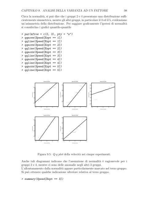
Circa la normalità, si può dire che i gruppi 2 e 4 presentano una distribuzione sufficientemente
simmetrica, mentre gli altri gruppi, in particolare il 3 ed il 5, evidenziano
un’asimmetria della distribuzione. Per saggiare graficamente l’ipotesi di normalità
si considerino i grafici quantile-quantile
> par(mfrow = c(2, 3), pty = "s")
> qqnorm(Speed[Expt == 1])
> qqline(Speed[Expt == 1])
> qqnorm(Speed[Expt == 2])
> qqline(Speed[Expt == 2])
> qqnorm(Speed[Expt == 3])
> qqline(Speed[Expt == 3])
> qqnorm(Speed[Expt == 4])
> qqline(Speed[Expt == 4])
> qqnorm(Speed[Expt == 5])
> qqline(Speed[Expt == 5])
Sample Quantiles
Sample Quantiles
700 800 900 1000
750 800 850 900
●
●
●
●
● ●
Normal Q−Q Plot
●
●
● ●
● ●
●
● ● ●
● ● ●
−2 −1 0 1 2
●
●
●
● ●
●
Theoretical Quantiles
Normal Q−Q Plot
●
●
● ●
● ●
−2 −1 0 1 2
●
●
● ●
Theoretical Quantiles
●
●
●
●
●
Sample Quantiles
Sample Quantiles
800 850 900 950
750 800 850 900 950
●
●
●
● ● ●
Normal Q−Q Plot
●
● ●
●
●
● ● ● ●
●
● ●
−2 −1 0 1 2
●
●
●
●
●
Theoretical Quantiles
Normal Q−Q Plot
● ● ● ● ● ●
●
●
●
● ● ●
−2 −1 0 1 2
Theoretical Quantiles
●
●
●
●
●
Sample Quantiles
650 700 750 800 850 900 950
●
● ●
Normal Q−Q Plot
● ● ● ●
●
● ●
● ●
● ● ● ● ●
−2 −1 0 1 2
Theoretical Quantiles
Figura 9.5: Q-q plot della velocità nei cinque esperimenti.
Anche tali diagrammi indicano che l’assunzione di normalità è ragionevole per i
gruppi 2 e 4, mentre ci sono delle anomalie negli altri 3 gruppi.
L’allontanamento dalla normalità appare particolarmente marcato nel terzo gruppo.
Si può ottenere qualche indicazione ulteriore relativa al terzo gruppo.
> summary(Speed[Expt == 3])
●
●
●