- Page 1 and 2: Practical Ship Hydrodynamics
- Page 3 and 4: Butterworth-Heinemann Linacre House
- Page 5 and 6: 3 Resistance and propulsion .......
- Page 7 and 8: 5.4.5 Interaction of rudder and shi
- Page 9 and 10: Preface The first five chapters giv
- Page 11 and 12: 1 Introduction Models now in tanks
- Page 13 and 14: Introduction 3 certain investigatio
- Page 15 and 16: Introduction 5 there have been prop
- Page 17 and 18: Introduction 7 is a material consta
- Page 19 and 20: Introduction 9 margin may make a di
- Page 21 and 22: Introduction 11 solution either. Ev
- Page 23 and 24: Introduction 13 in naval architectu
- Page 25 and 26: Introduction 15 ž Finite differenc
- Page 27 and 28: Introduction 17 makes seakeeping pr
- Page 29 and 30: Introduction 19 ship. Inner flow co
- Page 31 and 32: Introduction 21 performed on workst
- Page 33 and 34: Introduction 23 experts, while boun
- Page 35 and 36: Introduction 25 two more decades be
- Page 37 and 38: Introduction 27 Figure 1.3 A cylind
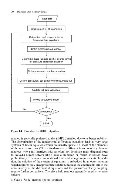
- Page 39: Introduction 29 resolved by conside
- Page 43 and 44: Introduction 33 flow direction. CDS
- Page 45 and 46: Introduction 35 equation, i.e. the
- Page 47 and 48: 2 Propellers 2.1 Introduction Ships
- Page 49 and 50: Propellers 39 ž rake iG The face o
- Page 51 and 52: KT KQ h 10 . K Q K T Figure 2.3 Pro
- Page 53 and 54: Propellers 43 methods or panel meth
- Page 55 and 56: Propellers 45 This formula can be i
- Page 57 and 58: Propellers 47 power. The earliest l
- Page 59 and 60: Propellers 49 corrected subsequentl
- Page 61 and 62: Propellers 51 flow computations are
- Page 63 and 64: Propellers 53 occurs earlier, as ca
- Page 65 and 66: Propellers 55 2.5.2 Open-water test
- Page 67 and 68: Propellers 57 the traditional prope
- Page 69 and 70: Propellers 59 (model/full-scale shi
- Page 71 and 72: Propellers 61 represents the cavity
- Page 73 and 74: Resistance and propulsion 63 1. The
- Page 75 and 76: Resistance and propulsion 65 3.1.2
- Page 77 and 78: Figure 3.3 Double-body flow y Wave
- Page 79 and 80: Resistance and propulsion 69 course
- Page 81 and 82: Resistance and propulsion 71 limite
- Page 83 and 84: Table 3.1 Recommended values for CA
- Page 85 and 86: Resistance and propulsion 75 3.2.6
- Page 87 and 88: P B ⋅ 10 3 (kW) 40 30 20 10 0 n P
- Page 89 and 90: Resistance and propulsion 79 t is t
- Page 91 and 92:
Resistance and propulsion 81 are no
- Page 93 and 94:
3.4 Simple design approaches Resist
- Page 95 and 96:
Resistance and propulsion 85 of the
- Page 97 and 98:
Resistance and propulsion 87 non-li
- Page 99 and 100:
Resistance and propulsion 89 resist
- Page 101 and 102:
Resistance and propulsion 91 (doubl
- Page 103 and 104:
Resistance and propulsion 93 only b
- Page 105 and 106:
Resistance and propulsion 95 resist
- Page 107 and 108:
Resistance and propulsion 97 1°. S
- Page 109 and 110:
Ship seakeeping 99 3. Addition of t
- Page 111 and 112:
Ship seakeeping 101 1. No recording
- Page 113 and 114:
Ship seakeeping 103 Re denotes the
- Page 115 and 116:
Ship seakeeping 105 the ship axis x
- Page 117 and 118:
Ship seakeeping 107 The procedure t
- Page 119 and 120:
Ship seakeeping 109 If several ω r
- Page 121 and 122:
a 0.015 0.010 0.005 0 1 2 3 4 5 Uc/
- Page 123 and 124:
Ship seakeeping 113 The (only stati
- Page 125 and 126:
Ship seakeeping 115 height H1/3 for
- Page 127 and 128:
Ship seakeeping 117 using data of B
- Page 129 and 130:
Ship seakeeping 119 for each strip
- Page 131 and 132:
Ship seakeeping 121 between near fi
- Page 133 and 134:
Ship seakeeping 123 wave length of
- Page 135 and 136:
Ship seakeeping 125 The elements of
- Page 137 and 138:
Ship seakeeping 127 4.4.3 Rankine s
- Page 139 and 140:
Ship seakeeping 129 to zero. Then t
- Page 141 and 142:
Ship seakeeping 131 for commercial
- Page 143 and 144:
Ship seakeeping 133 Since the spect
- Page 145 and 146:
Ship seakeeping 135 ž The ωj are
- Page 147 and 148:
Ship seakeeping 137 changing sea sp
- Page 149 and 150:
Ship seakeeping 139 The wave impact
- Page 151 and 152:
Ship seakeeping 141 pressure gauges
- Page 153 and 154:
v(t) h(x,t) y u(x,t) Figure 4.23 On
- Page 155 and 156:
Ship seakeeping 145 computations wi
- Page 157 and 158:
Ship seakeeping 147 4. Derive the p
- Page 159 and 160:
Ship seakeeping 149 The free consta
- Page 161 and 162:
5 Ship manoeuvring 5.1 Introduction
- Page 163 and 164:
Ship manoeuvring 153 ž yaw rate (r
- Page 165 and 166:
Ship manoeuvring 155 Table 5.2 Non-
- Page 167 and 168:
Ship manoeuvring 157 but also the i
- Page 169 and 170:
C y 1.50 1.25 1.00 1.75 0.85 0.80 0
- Page 171 and 172:
Ship manoeuvring 161 section. The l
- Page 173 and 174:
Ship manoeuvring 163 methods have b
- Page 175 and 176:
esistance R is proportional to spee
- Page 177 and 178:
Ship manoeuvring 167 accuracy, but
- Page 179 and 180:
Ship manoeuvring 169 the difference
- Page 181 and 182:
Ship manoeuvring 171 it is importan
- Page 183 and 184:
d, y 20° 10° 0° −10° −20°
- Page 185 and 186:
Distance Lateral deviation Length o
- Page 187 and 188:
Ship manoeuvring 177 also performed
- Page 189 and 190:
Ship manoeuvring 179 ž Rudders out
- Page 191 and 192:
ehind the leading edge (nose) is: c
- Page 193 and 194:
Ship manoeuvring 183 the rudder. In
- Page 195 and 196:
Ship manoeuvring 185 attack ˛ of n
- Page 197 and 198:
V a /V 0.4 0.3 0.2 0.1 V a /V 2.0 1
- Page 199 and 200:
Ship manoeuvring 189 ž Rudder with
- Page 201 and 202:
average between VA and V1: � �
- Page 203 and 204:
C L (V corr ≠ V A ) C L (V corr =
- Page 205 and 206:
Ship manoeuvring 195 hull influence
- Page 207 and 208:
Ship manoeuvring 197 - Estimate the
- Page 209 and 210:
Ship manoeuvring 199 rudder tip vor
- Page 211 and 212:
Ship manoeuvring 201 (1993) uses de
- Page 213 and 214:
Ship manoeuvring 203 ž Profiles wi
- Page 215 and 216:
Ship manoeuvring 205 The ship perfo
- Page 217 and 218:
6 Boundary element methods 6.1 Intr
- Page 219 and 220:
C ⊲t1n3 C n1t3⊳⊲t3 xxz C s3 x
- Page 221 and 222:
xx D ⊲ 3 x⊲x xq⊳ ⊳/r 2 xy D
- Page 223 and 224:
The velocity in the x direction is:
- Page 225 and 226:
∂ ∂z Boundary element methods 2
- Page 227 and 228:
Boundary element methods 217 2. Thr
- Page 229 and 230:
and ⊲ , ⊳ is: r D � ⊲x ⊳
- Page 231 and 232:
⊲1⊳ y D � d 2 y d r 2 f ⊲c
- Page 233 and 234:
Boundary element methods 223 the so
- Page 235 and 236:
2 0 8xz D 2 2 0 8xxz D 2 2 0 8xzz D
- Page 237 and 238:
Figure 6.9 Velocities induced by po
- Page 239 and 240:
It is convenient to write ϕ as:
- Page 241 and 242:
Boundary element methods 231 usuall
- Page 243 and 244:
Boundary element methods 233 From t
- Page 245 and 246:
with: Boundary element methods 235
- Page 247 and 248:
Numerical example for BEM 237 S is
- Page 249 and 250:
Numerical example for BEM 239 In ea
- Page 251 and 252:
Numerical example for BEM 241 Once
- Page 253 and 254:
Numerical example for BEM 243 ž Tr
- Page 255 and 256:
Numerical example for BEM 245 that
- Page 257 and 258:
Numerical example for BEM 247 is ch
- Page 259 and 260:
Table 7.1 Sign for derivatives of p
- Page 261 and 262:
z y Figure 7.5 Coordinate system us
- Page 263 and 264:
the contour (Fig. 7.5): n� iD1 i
- Page 265 and 266:
Numerical example for BEM 255 Let E
- Page 267 and 268:
Numerical example for BEM 257 At th
- Page 269 and 270:
Numerical example for BEM 259 This
- Page 271 and 272:
Numerical example for BEM 261 The i
- Page 273 and 274:
Numerical example for BEM 263 The e
- Page 275 and 276:
References Abbott, I. and Doenhoff,
- Page 277 and 278:
References 267 Morgan, W. B. and Li
- Page 279 and 280:
Index Actuator disk, 44 Added mass,