N=2 Supersymmetric Gauge Theories with Nonpolynomial Interactions

More documents

Recommendations

Info

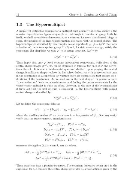
12 Chapter 1. Gauging the Central Charge 1.3 The Hypermultiplet A simple yet instructive example for a multiplet with a nontrivial central charge is the massive Fayet-Sohnius hypermultiplet [8, 4]. Although it contains no gauge fields by itself, we shall nevertheless demonstrate, as a warm-up for more complicated things to come, the gauging of the rigid transformation associated with the central charge. The hypermultiplet is described by two complex scalar superfields ϕ i , ¯ϕi = (ϕ i ) ∗ that form a doublet of the automorphism group SU(2) and, for rigid central charge, satisfy the constraints (for simplicity we take ϕ i to be gauge invariant, δIϕ i = 0) D (i α ϕ j) = 0 = ¯ D (i ˙α ϕj) . (1.49) These imply that only ϕ i itself contains independent components, while those of the central charge images ϕ i(z) , etc. can be expressed in terms of the ones of ϕ i and derivatives thereof. It is now a fundamental question whether, upon gauging the central charge, it suffices to simply replace the flat spinor derivatives with gaugecovariant ones in the constraints on a superfield, or whether there are obstructions that require modifications of the constraints. As we shall see in the next chapter, in general a naive “covariantization” leads to inconsistencies, and finding the proper constraints for the vector-tensor multiplet is quite an effort. However, in the case of the hypermultiplet it turns out that the first attempt is successful, i.e. the hypermultiplet with gauged central charge is described by Let us define the component fields as D (i αϕ j) = 0 = ¯ D (i ˙α ϕj) . (1.50) ϕ i | , χ α = 1 2 Dαiϕ i | , ¯ ψ ˙α = 1 2 ¯ D ˙αiϕ i | , F i = δzϕ i | , (1.51) where the auxiliary scalars F i do occur also in a θ-expansion of ϕ i . One may easily verify that the supersymmetry transformations D i αϕ j = ε ijχ α , D i α ¯ϕ j = −ε ij ψα D i α χ β = −εαβ ¯ ZF i , D i α ¯χ ˙α = −i Dα ˙α ¯ϕ i D i α ¯ ψ ˙α = −i Dα ˙αϕ i , D i αψβ = εαβ ¯ Z ¯ F i D i αF j = ε ij δz χ α , D i α ¯ F j = −ε ij δzψα represent the algebra (1.33) when δz acts as follows, δzχα = − 1 µ iσ Dµ Z ¯ ψ + λiF i α , δz ¯ ψ ˙α = − 1 iDµ Z¯ χσ µ + ¯ λiF i ˙α δzF i = 1 |Z| 2 µ D Dµϕ i + λ i δzχ + ¯ λ i δz ¯ ψ − Y ij Fj . (1.52) (1.53) These equations have a peculiar structure. The covariant derivative acting on ¯ ψ in the expression for δz χ contains the central charge generator δz, whose action is given by the
1.3. The Hypermultiplet 13 second equation, which in turn involves a covariant derivative of χ. Hence, the central charge transformation of χ is given only implicitly as the equations are coupled. Let us insert the second one into the first, |Z| 2 δz χ α = −iAα ˙α ¯ Zδz ¯ ψ ˙α − ¯ Z(i∂α ˙α ¯ ψ ˙α + λαiF i ) = −iAα ˙α(iD ˙αβχ β − ¯ λ ˙α i F i ) − ¯ Z(i∂α ˙α ¯ ψ ˙α + λαiF i ) = Aα ˙αA ˙αβ δz χ β + Aα ˙α(∂ ˙αβχ β + i ¯ λ ˙α i F i ) − ¯ Z(i∂α ˙α ¯ ψ ˙α + λαiF i ) . According to eq. (A.23) Aα ˙αA ˙αβ = A µ Aµδ β α, so we have isolated δz χ α. Doing a similar calculation for ¯ ψ, we conclude that where the abbreviation δzχα = − 1 iZ(∂α ¯ ˙α E ¯ ψ ˙α − iλαiF i ) − Aα ˙α(∂ ˙αβχβ + i¯ λ ˙α i F i ) δz ¯ ψ ˙α = − 1 iZ(∂α ˙α E χα − i¯ λ ˙αiF i ) − Aα ˙α(∂ ˙ βα ψ¯ β ˙ + iλ α i F i ) , E ≡ |Z| 2 − A µ Aµ (1.54) (1.55) has been introduced. Since Z has a nonvanishing vev, E may be inverted at least formally. We can restructure the central charge transformation of F i in like manner, for the covariant d’Alembertian acting on ϕ i may be expanded as Thus one finds D µ Dµϕ i = ϕ i + F i ∂µA µ + 2A µ ∂µF i + A µ AµδzF i . δzF i = 1 i i ϕ + F ∂µA E µ + 2A µ ∂µF i + λ i δzχ + ¯ λ i δz ¯ ψ − Y ij Fj . (1.56) Note that in the limit Z = i, which corresponds to a rigid central charge, the transformations reduce to δz χ = −σ µ ∂µ ¯ ψ , δz ¯ ψ = −¯σ µ ∂µ χ , δzF i = ϕ i , (1.57) hence in the massless case they are trivial on-shell (cf. the Lagrangian given below). In order to determine an invariant action, we apply the prescription (1.42) derived in the previous section. The constraints (1.50) imply that the combinations L ij ↔ (i 0 = − ¯ϕ δzϕ j) , L ij m = −2i m ¯ϕ (i ϕ j) , m ∈ R (1.58) are both linear superfields, thus giving rise to two independent invariants. Let us consider the first; a straightforward computation leads to L0 = − 1 2 ¯ϕiD µ Dµϕ i − 1 2 ϕiD µ Dµ ¯ϕi − i ↔ χσ µ Dµ 2 ¯χ ↔ µ + ψσ Dµ ¯ ψ + |Z| 2 F i Fi ¯ + 1 2 Aµ i ϕ ↔ D µ ↔ Fi ¯ + ¯ϕi D µ F i ↔ µ + iχσ δz ¯χ ↔ µ + iψσ δz ¯ ψ . (1.59)
Page 1 and 2: N=2 Supersymmetric Gauge Theories w
Page 3: Abstract In this thesis the central
Page 6 and 7: Acknowledgments I would like to exp
Page 9 and 10: Introduction Despite the lack of ex
Page 11 and 12: Chapter 1 Gauging the Central Charg
Page 13 and 14: 1.1. The N=2 Supersymmetry Algebra
Page 15 and 16: 1.1. The N=2 Supersymmetry Algebra
Page 17 and 18: 1.2. The Linear Multiplet 9 1.2 The
Page 19: 1.2. The Linear Multiplet 11 It wil
Page 23: 1.3. The Hypermultiplet 15 so in th
Page 26 and 27: 18 Chapter 2. The Vector-Tensor Mul
Page 45 and 46: Chapter 3 The Linear Case In this c
Page 47 and 48: 3.2. Transformations and Bianchi Id
Page 53 and 54: 3.3. The Lagrangian 45 7) 0 = ∂
Page 55 and 56: 3.3. The Lagrangian 47 compute the
Page 57 and 58: 3.4. Chern-Simons Couplings 49 To c
Page 59 and 60: 3.4. Chern-Simons Couplings 51 Here
Page 61 and 62: 3.5. Henneaux-Knaepen Models 53 eq.
Page 63 and 64: 3.5. Henneaux-Knaepen Models 55 whe
Page 65 and 66: Chapter 4 The Nonlinear Case In sec
Page 71 and 72:
4.2. Transformations and Bianchi Id
Page 73 and 74:
4.3. The Lagrangian 65 This of cour
Page 75:
4.3. The Lagrangian 67 which introd
Page 78 and 79:
70 Conclusions and Outlook likely t
Page 80 and 81:
72 Appendix A. Conventions and the
Page 82 and 83:
74 Appendix A. Conventions σ µν
Page 84 and 85:
76 References [20] N. Dragon and S.
show all

N=2 Supersymmetric Gauge Theories with Nonpolynomial Interactions

You also want an ePaper? Increase the reach of your titles

Delete template?

Save as template?