N=2 Supersymmetric Gauge Theories with Nonpolynomial Interactions

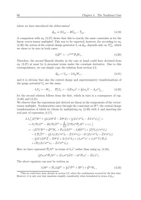
60 Chapter 4. The Nonlinear Case
where we have introduced the abbreviation 1
Gµν ≡ IGµν − R ˜ Gµν − ˜ Σµν . (4.19)
A comparison with eq. (3.27) shows that this is exactly the same constraint as for the
linear vector-tensor multiplet! This was to be expected, however, for according to eq.
(2.36) the action of the central charge generator δz on Gµν depends only on N ij
α ˙α , which
we chose to be zero in both cases,
δz ˜ G µν = −ε µνρσ DρWσ . (4.20)
Therefore, the second Bianchi identity in the case at hand could have deviated from
eq. (3.27) at most by δz-invariant terms under the covariant derivative. Due to this
correspondence, we can simply copy the solution from section 3.2,
Gµν = Vµν − 2A[µWν] , (4.21)
and it is obvious that also the central charge and supersymmetry transformations of
the gauge potential Vµ are the same,
δzVµ = −Wµ , D i αVµ = − i ¯ Zσµ ¯ ψ i + 1
2Lσµ ¯ λ i − Aµψ i
, (4.22)
α
for the second relation follows from the first, which in turn is a consequence of eqs.
(4.20) and (4.21).
We observe that the expressions just derived are linear in the components of the vectortensor
multiplet. Nonlinearities enter through the constraint on W µ , the central charge
transformation of which we obtain by multiplying eq. (2.39) with L and inserting the
real part of expression (4.17),
2 µ i
L δz |Z| W + 2L(Z∂µ Z¯ − Z∂ ¯ µ i Z) + 2 (Zψiσ µ¯ λi − ¯ Zλ i σ µ ψi) ¯ =
= IL DνG µν − RL Dν ˜ G µν + L
Z Diσ
12
µ DjM ¯ ij + c.c.
= −|Z| 2 UW µ + ˜ G µν Wν + Dν(LIG µν − LR ˜ G µν ) + |Z| 2 δz(ψ i σ µ ψi) ¯
− L Dν ˜ Σ µν − i
2 L δz(Zψ i σ µ¯ λi − ¯ Zλ i σ µ ¯ ψi) − iU(Zψ i σ µ¯ λi − ¯ Zλ i σ µ ¯ ψi)
− i
2 LU(Z∂µ ¯ Z − ¯ Z∂ µ Z + 2i λ i σ µ¯ λi) + (λiσ µν ψ i + ¯ ψi¯σ µν ¯ λ i ) DνL
+ i Dν(Zψ i σ µν ψi − ¯ Z ¯ ψ i ¯σ µν ¯ ψi) .
Here we have expressed ¯ DjM ij in terms of δz ¯ ψ i rather than using eq. (4.16),
i
3Zψiσ µ DjM ¯ ij = Zψiσ µ (i¯ λ i U − i¯σ ν Dνψ i − ¯ Zδz ¯ ψ i ) .
The above equation can now be written as
δzW µ = Dν(LG µν + 1
2 L2 ˜ F µν + Π µν ) + ˜ G µν Wν , (4.23)
1 This we could have done already in section 2.2, where the combination occured for the first time.
However, it is only now that equations simplify considerably when formulated in terms of Gµν.