N=2 Supersymmetric Gauge Theories with Nonpolynomial Interactions

More documents

Recommendations

Info

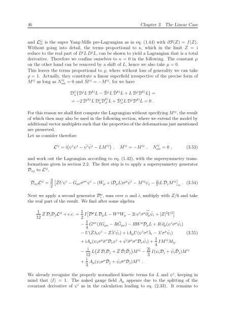
46 Chapter 3. The Linear Case and L ij cc is the super Yang-Mills pre-Lagrangian as in eq. (1.44) with ∂F(Z) = f(Z). Without going into detail, the terms proportional to κ, which in the limit Z = i reduce to the real part of D i L D j L, can be shown to yield a Lagrangian that is a total derivative. Therefore we confine ourselves to κ = 0 in the following. The constant µ on the other hand can be removed by a shift of L, hence we also take µ = 0. This leaves the terms proportional to ϱ, where without loss of generality we can take ϱ = 1. Actually, they constitute a linear superfield irrespective of the precise form of M ij as long as N ij α ˙α = 0 and ¯ M ij = −M ij , for we have D (i j k) α D L D L − D¯ j L D¯ k) j k) L + L D D L = = −2 D β(i L D j αD k) β L + D(i αL D j D k) L = 0 . For this reason we shall first compute the Lagrangian without specifying M ij , the result of which then may also be used in the following section, where we extend the model by additional vector multiplets such that the properties of the deformations just mentioned are preserved. Let us consider therefore L ij = i ψ i ψ j − ¯ ψ i ψ¯ j ij − LM , M¯ ij ij ij = −M , Nα ˙α = 0 , (3.53) and work out the Lagrangian according to eq. (1.42), with the supersymmetry transformations given in section 2.2. The first step is to apply a supersymmetry generator Dαj to L ij , DαjL ij = 3 2 ¯ZUψ i − Gµνσ µν ψ i − (Wµ + iDµL)σ µ ψ¯ i ij − M ψj − 2iL DjM ij . (3.54) 3 α Next we apply a second generator D α i , sum over α and i, multiply with Z/6 and take the real part of the result. We find after some algebra 1 12 Z DiDjL ij + c.c. = 1 2 ID µ L DµL − W µ Wµ − 2i ψ i ↔ µ σ ∂µ ¯ ψi + |Z| 2 U 2 − 1 4 Gµν (IGµν − R ˜ Gµν) − RW µ DµL + R ∂µ(ψ i σ µ ψi) ¯ − U( ¯ Zλiψ i − Z¯ λ i ψi) ¯ + iAµU(ψ i σ µ¯ λi − λ i σ µ ψi) ¯ (3.55) + iAµ(ψiσ µ ¯σ ν Dνψ i + ¯ ψ i ¯σ µ σ ν Dν ¯ ψi) + 1 4 IM ij Mij − i 12 LZ DiDj + ¯ Z ¯ Di ¯ ij 2i Dj M − 3 I(ψiDj + ¯ ψi ¯ Dj)M ij + i 3 Aµ(ψiσ µ Dj ¯ + ¯ ψi¯σ µ Dj)M ij . We already recognize the properly normalized kinetic terms for L and ψ i , keeping in mind that 〈I〉 = 1. The naked gauge field Aµ appears due to the splitting of the covariant derivative of ψ i as in the calculation leading to eq. (2.33). It remains to
3.3. The Lagrangian 47 compute the mixed derivative of L ij that couples to Aµ in eq. (1.42). It reads i 6 AµDiσ µ ¯ DjL ij = RUAµW µ − IUAµD µ L − G µν AµWν + ˜ G µν Aµ∂νL − iAµ(ψiD µ ψ i + ¯ ψ i D µ ¯ ψi) − i 3 Aµ(ψiσ µ ¯ Dj + ¯ ψi¯σ µ Dj) M ij + 1 6 LAµ Diσ µ ¯ DjM ij , (3.56) and we observe that the terms in the second line cancel the corresponding ones in the previous equation. While in general M ij has to be specified before the action of the supersymmetry generators can be computed, the last term in eq. (3.56) may be simplified by virtue of the Bianchi identity (BI.2). Since by assumption M ij = 0, one has is imaginary and N ij α ˙α 1 6 LAµ Diσ µ DjM ¯ ij = 1 I AµL I ∂ν ˜ G µν + R ∂νG µν + 1 2U∂µ |Z| 2 + 1 2 δz(Zψ i σ µ¯ λi + ¯ Zλ i σ µ ¯ ψi) . (3.57) The effect of the terms (3.56) is twofold; first they introduce the anticipated coupling of the current (2.16) to the gauge field Aµ (contained in the term G µν AµWν, see below), and second they reduce the covariant derivatives to partial ones, similar to the case of the hypermultiplet (cf. L0 in eq. (1.59)). One finds for instance D µ L DµL − 2UAµD µ L = ∂ µ L ∂µL − A µ AµU 2 . The resulting Lagrangian eventually reads L = 1 2 I∂ µ L ∂µL − W µ Wµ − 2i ψ i ↔ µ σ ∂µ ¯ ψi + EU 2 + R − 1 4 Gµν IGµν − R ˜ Gµν + 4AµWν I LAµ∂νG µν + LM + W µ Λµ + 1 2 ˜ G µν Σµν − W µ ∂µ(LR) + 1 2I LUAµ ∂µ|Z| 2 − i 2 ∂µL (ψ i σ µ¯ λi − λ i σ µ ¯ ψi) + i 2 Yij(ψ i ψ j − ¯ ψ i ¯ ψ j ) (3.58) − 1 2 U( ¯ Zλiψ i − Z¯ λ i ψi) ¯ + i 2 AµU(ψ i σ µ¯ λi − λ i σ µ ψi) ¯ + R ∂µ(ψ i σ µ ψi) ¯ + i 2 Fµν(ψiσ µν ψ i + ¯ ψ i ¯σ µν ψi) ¯ + 1 2I LAµ δz(Zψ i σ µ¯ λi + ¯ Zλ i σ µ ψi) ¯ LG ˜µν Aν + iAν(ψiσ µν ψ i + ¯ ψ i ¯σ µν ψi) ¯ , − ∂µ where the part LM = − i 12 LZ DiDjM ij − i 3 (Lλi + 2Iψi)DjM ij + 1 8 − 1 λiψj − 4 ¯ λi ¯ ij ψj + iLYij M + c.c. IMijM ij (3.59) has to be determined separately for each model, which however is easy as all the terms have been computed already for the Bianchi identities.
Page 1 and 2:
N=2 Supersymmetric Gauge Theories w
Page 3: Abstract In this thesis the central
Page 6 and 7: Acknowledgments I would like to exp
Page 9 and 10: Introduction Despite the lack of ex
Page 11 and 12: Chapter 1 Gauging the Central Charg
Page 13 and 14: 1.1. The N=2 Supersymmetry Algebra
Page 15 and 16: 1.1. The N=2 Supersymmetry Algebra
Page 17 and 18: 1.2. The Linear Multiplet 9 1.2 The
Page 19 and 20: 1.2. The Linear Multiplet 11 It wil
Page 21 and 22: 1.3. The Hypermultiplet 13 second e
Page 23: 1.3. The Hypermultiplet 15 so in th
Page 26 and 27: 18 Chapter 2. The Vector-Tensor Mul
Page 45 and 46: Chapter 3 The Linear Case In this c
Page 47 and 48: 3.2. Transformations and Bianchi Id
Page 53: 3.3. The Lagrangian 45 7) 0 = ∂
Page 57 and 58: 3.4. Chern-Simons Couplings 49 To c
Page 59 and 60: 3.4. Chern-Simons Couplings 51 Here
Page 61 and 62: 3.5. Henneaux-Knaepen Models 53 eq.
Page 63 and 64: 3.5. Henneaux-Knaepen Models 55 whe
Page 65 and 66: Chapter 4 The Nonlinear Case In sec
Page 73 and 74: 4.3. The Lagrangian 65 This of cour
Page 75: 4.3. The Lagrangian 67 which introd
Page 78 and 79: 70 Conclusions and Outlook likely t
Page 80 and 81: 72 Appendix A. Conventions and the
Page 82 and 83: 74 Appendix A. Conventions σ µν
Page 84 and 85: 76 References [20] N. Dragon and S.
show all

N=2 Supersymmetric Gauge Theories with Nonpolynomial Interactions

Create successful ePaper yourself

Delete template?

Save as template?