N=2 Supersymmetric Gauge Theories with Nonpolynomial Interactions

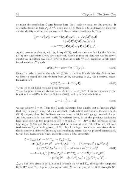
52 Chapter 3. The Linear Case
contains the nonabelian Chern-Simons form that lends its name to this section. It
originates from the term F I µν ˜ F µνI , which can be written as a total derivative using the
Jacobi identity and the antisymmetry of the structure constants fIJ K δKL,
1
2 εµνρσF I µνF I ρσ = 2ε µνρσ ∂ µA I ν ∂ρA I σ − fJK I A J µA K ν ∂ρA I σ
+ 1
4AJ µA K ν A L ρ A M σ fJK I fLM I
I
Aν∂ρA I σ − 1
= 2ε µνρσ ∂µ
3 AI νA J ρ A K σ fJK I .
Again, one can replace Λµ with ˆ Λµ in eq. (3.29), and we conclude that for the function
(3.78) the constraints (3.67) are consistent, since the Bianchi identities can be solved
exactly as in section 3.2. Note however that, although ˆ Λ µ is δI-invariant, a full gauge
transformation ∆ g yields
∆ g (C) ˆ Λ µ = 2e ε µνρσ ∂ν(C I ∂ ρA I σ) . (3.81)
Hence, in order to render the solution (3.30) to the first Bianchi identity ∆ g -invariant,
we have to cancel the contribution from ˆ Λ µ by assigning to Bµν the nontrivial transformation
law
∆ g (C) Bµν = −4e C I ∂ [µA I ν] . (3.82)
Vµ on the other hand remains gauge invariant.
What happens when we choose eφ = Z, i.e. F = Z 2 /2e? This corresponds to the
function h = −2iZ/e in the coefficients (3.66), and by a field redefinition
L = ˆ L + i e (Z − ¯ Z) (3.83)
we can achieve ˆ h = 0. Thus the Bianchi identities have singled out a function F(Z)
that may be gauged away, which shows that, modulo field redefintions, the constraints
(3.19) uniquely describe the linear vector-tensor multiplet with gauged central charge.
An invariant action can now easily be written down, as in the previous section we
have used only the two properties N ij
α ˙α = 0 and ¯ M ij = −M ij in the derivation of the
Lagrangian (3.58), and these are also valid in the case at hand. Therefore, we just need
to determine LM according to eq. (3.59). As all the ingredients have been given above,
this is merely a matter of inserting and combining terms, and we proceed immediately
to the final Lagrangian, which reads (modulo a total derivative)
µ
L = LlinVT Λ → Λ ˆ µ
, Σµν → ˆ
Σµν + Lcc
− 2e iF I µνψiσ µνχ iI − ψ i σ µ ¯χ I
i Dµ ¯ φ I + (φ − ¯ φ) I ψ i σ µ Dµ ¯χI
i + iD ijI ψi χI j
+ i
2 ψiχ J i ¯ φ K fJK I φ I + c.c. − e ∂µL (φ + ¯ φ) I ∂ µ (φ + ¯ φ) I
+ (eL + 1/4g 2 ) 2D µ φ I Dµ ¯ φ I − F µνI F I µν − iχiI ↔
µ
σ Dµ ¯χI
+ χ iIχ J i ¯ φ K − ¯χ I
i ¯χiJ φ K fJK I + 1
2
i + D I ijD ijI
φ J ¯ φ K fJK I 2 .
(3.84)
LlinVT has been given in eq. (3.61) and depends on Λ µ and Σµν through the composite
fields W µ and Gµν. Upon replacing Λ µ with ˆ Λ µ in the generalized field strength H µ ,