N=2 Supersymmetric Gauge Theories with Nonpolynomial Interactions

More documents

Recommendations

Info

54 Chapter 3. The Linear Case Comparing with section 2.1, we observe that the δa generalize the rigid central charge transformations of the free vector-tensor multiplet. When more than one antisymmetric tensor is considered, there are also nontrivial second-order currents J µνA = 1 2 fBC A ε µνρσ H B ρ H C σ , (3.92) which are conserved on-shell for any constants fAB C = f[AB] C , but do not correspond to any global symmetry of L. Henneaux and Knaepen have been able to simultaneously deform the free action (3.89) and the gauge transformations (3.88) such that the symmetries generated by the δa are realized locally. At first order in the deformation parameter g the gauge fields couple to the respective currents, giving rise to so-called Freedman-Townsend vertices. At second order in g a condition arises on the as yet arbitrary constants T a A b and fAB C , namely the fAB C have to satisfy a Jacobi identity, which identifies them as structure constants of a Lie algebra, while the matrices TA are required to define a real representation of the same, f[AB D fC]D E = 0 , [ TA , TB ] = fAB C TC . (3.93) It is possible, and convenient, to present the resulting model in a first order formulation, where the Lagrangian and the transformations are polynomial. To this end, we introduce auxiliary vector fields W A µ , which may be eliminated later on to obtain the nonpolynomial form. The complete Lagrangian then reads LHK = − 1 4 εµνρσW A µνBρσA − 1 4 FµνaδabF b µν + cab ˜ F b 1 µν + 2 δABW µA W B µ , (3.94) where cab ∈ R and W A µν = ∂µW A ν − ∂ νW A µ + gfBC A W B µ W C ν (3.95) F a µν = ∇µA a ν − ∇νA a µ , ∇µA a ν = ∂µA a ν + gW A µ T a A bA b ν . (3.96) W A µν resembles a nonabelian Yang-Mills field strength, in particular it satisfies the Bianchi identity ε µνρσ ∇νW A ρσ = ε µνρσ (∂νW A µν + gW B ν fBC A W C ρσ) = 0 , (3.97) but due to the presence of the last term in LHK there is no gauge transformation associated with W A µ that leaves LHK invariant. The term proportional to the constants cab, which may be chosen arbitrarily, slightly extends the original model of Henneaux and Knaepen. As we shall see, it gives rise to Chern-Simons couplings, which however neither include the nonabelian ones of the previous section, nor do they describe the nonlinearities of the self-interacting vector-tensor multiplet we are going to construct in the following chapter. This suggests that the Henneaux-Knaepen models presented here admit a further generalization. The conditions (3.93) are sufficient 3 to render d 4 x LHK invariant under the following two sets of gauge transformations: First one may vary just the BµνA, ∆ B (Ω) BµνA = −2 ∇[µΩν]A , ∆ B (Ω) A a µ = 0 , ∆ B (Ω) W A µ = 0 , (3.98) 3 We emphasize that the Lie algebra need not be compact and that the metrics δab, δAB as well as the constants cab need not be invariant tensors.
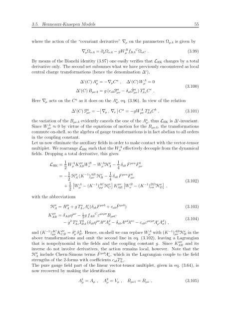
3.5. Henneaux-Knaepen Models 55 where the action of the “covariant derivative” ∇µ on the parameters ΩµA is given by ∇µΩνA = ∂µΩνA − gW B µ fBA C ΩνC . (3.99) By means of the Bianchi identity (3.97) one easily verifies that LHK changes by a total derivative only. The second set subsumes what we have previously encountered as local central charge transformations (hence the denomination ∆ z ), ∆ z (C) A a µ = −∇µC a , ∆ z (C) W A µ = 0 ∆ z (C) BµνA = g (cabF a µν − δab ˜ F a µν) T b A cC c . Here ∇µ acts on the C a as it does on the A a µ, eq. (3.96). In view of the relation (3.100) ∆ z (C) F a µν = −[ ∇µ , ∇ν ] C a = −gW A µν T a A bC b , (3.101) the variation of the BµνA evidently cancels the one of the A a µ, thus LHK is ∆ z -invariant. Since W A µν ≈ 0 by virtue of the equations of motion for the BµνA, the transformations commute on-shell, so the algebra of gauge transformations is in fact abelian to all orders in the coupling constant. Let us now eliminate the auxiliary fields in order to make contact with the vector-tensor multiplet. We rearrange LHK such that the W A µ effectively decouple from the dynamical fields. Dropping a total derivative, this gives LHK = 1 2 W A µ K µν ABW B ν − W A µ H µ 1 A − 4 δab F µνa F b µν = − 1 µν H ν B − 1 2 Hµ + 1 2 with the abbreviations A (K−1 ) AB W A µ − (K −1 ) AC µρ H ρ C 4 δab F µνa F b µν K µν AB W B ν − (K −1 ) BD νσ H σ D , (3.102) H µ A = Hµ A + g T a A cA c ν(δabF µνb + cab ˜ F µνb ) (3.103) K µν AB = δABη µν − 1 2 g fAB C ε µνρσ BρσC − g 2 T a A cT b B d (δabη µν A ρc A d ρ − δabA µd A νc − cabε µνρσ A c ρA d σ) , (3.104) and (K−1 ) AC µρ K ρν CB = δν µ δA B . Hence, on-shell we can replace W A µ with (K−1 ) AB µν Hν B in the above transformations and omit the second line in eq. (3.102), leaving a Lagrangian that is nonpolynomial in the fields and the coupling constant g. Since K µν AB and its inverse do not involve derivatives, the action remains local, however. Note that the H µ A include Chern-Simons terms ˜ F µνbA c ν, which in the Lagrangian couple to the field strengths of the 2-forms with coefficients cabT a A c . The pure gauge field part of the linear vector-tensor multiplet, given in eq. (3.64), is now recovered by making the identification A 1 µ = Aµ , A 2 µ = Vµ , Bµν1 = Bµν , (3.105)
Page 1 and 2:
N=2 Supersymmetric Gauge Theories w
Page 3:
Abstract In this thesis the central
Page 6 and 7:
Acknowledgments I would like to exp
Page 9 and 10:
Introduction Despite the lack of ex
Page 11 and 12: Chapter 1 Gauging the Central Charg
Page 13 and 14: 1.1. The N=2 Supersymmetry Algebra
Page 15 and 16: 1.1. The N=2 Supersymmetry Algebra
Page 17 and 18: 1.2. The Linear Multiplet 9 1.2 The
Page 19 and 20: 1.2. The Linear Multiplet 11 It wil
Page 21 and 22: 1.3. The Hypermultiplet 13 second e
Page 23: 1.3. The Hypermultiplet 15 so in th
Page 26 and 27: 18 Chapter 2. The Vector-Tensor Mul
Page 45 and 46: Chapter 3 The Linear Case In this c
Page 47 and 48: 3.2. Transformations and Bianchi Id
Page 53 and 54: 3.3. The Lagrangian 45 7) 0 = ∂
Page 55 and 56: 3.3. The Lagrangian 47 compute the
Page 57 and 58: 3.4. Chern-Simons Couplings 49 To c
Page 59 and 60: 3.4. Chern-Simons Couplings 51 Here
Page 61: 3.5. Henneaux-Knaepen Models 53 eq.
Page 65 and 66: Chapter 4 The Nonlinear Case In sec
Page 73 and 74: 4.3. The Lagrangian 65 This of cour
Page 75: 4.3. The Lagrangian 67 which introd
Page 78 and 79: 70 Conclusions and Outlook likely t
Page 80 and 81: 72 Appendix A. Conventions and the
Page 82 and 83: 74 Appendix A. Conventions σ µν
Page 84 and 85: 76 References [20] N. Dragon and S.
show all

N=2 Supersymmetric Gauge Theories with Nonpolynomial Interactions

Create successful ePaper yourself

Delete template?

Save as template?