A Wavelength Converter Integrated with a Discretely Tunable Laser ...

More documents

Recommendations

Info

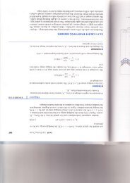
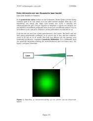
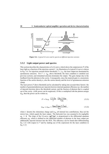
28 3. Semiconductor optical amplifier operation and device characterization [mW] P stimulated emmision spontaneous emmision Ith ΔI ΔP I wavelength wavelength spectral power Figure 3.6: A typical LI-curve and its spectra at different injection currents. 3.3.2 Light output power and spectra This section describes the characteristics of a LI-curve, which shows the output power of the laser light as a function of the injection current . An illustration of a typical LI-curve is shown in Fig. 3.6. For injection currents below threshold, £ , the laser output are dominated by spontaneous emission. For © , above threshold, the laser condition is satisfied (see previous section), and stimulated emission dominates the output. The gain clamps due to the feedback from the photons in the cavity. Consequently, since the material gain is a monotonic function of the carrier density , also the carrier density and the level of spontaneous emission clamp. The laser power above threshold can be calculated by taking into account three factors: the number of generated photons per injected electron (internal quantum efficiency ), the number of injected electrons above the threshold current, and the fraction of photons that is coupled out of the cavity. (ASE power can be neglected.) If this is multiplied with the photon energie then the power can be written as, ¡ (3.21) ¡ ¡ (3.22) ¡ where denotes the elementary charge ¡ and all internal loss contributions, thus not the mirror loss, which equals the laser output. The butt-joint loss was assumed to be negligible , is proportional to the differential quantum . The slope of the LI-curve, ¡ efficiency , which is defined as the additional number of photons in the laser output per additionally injected electron into the SOA. The efficiency can be found after differentiating Eq. 3.21 with respect to and by making use of the expression for the laser condition in Eq. 3.15:
3.3 Extended Cavity Lasers and extended waveguide SOAs 29 Inversion of Eq. 3.23 gives ¤ ¤ ¡ ¤ ¡ ¦ ¤ ¦ from which it can be seen that the reciprocal differential quantum efficiency linearly on the laser length , a relation which can be tested experimentally. ¤ (3.23) (3.24) depends Measured LI-curves from the ECL test structures are shown in Fig. 3.7. No coating was applied to the facets. The power on the vertical axis represents fiber coupled power (§ ¨ dB coupling loss). The emitted power from two facets for the 400 long laser is over 1.5 mW at ¤ mA. The curves show an almost linear increase in the output power with increasing current, as expected. From the curves we extracted the threshold current density, , and the differential quantum efficiency, , both as a function of , and compared them to the theory as is described below. Threshold current density The measured values of as a function of ¤ were fitted using Eq. 3.18 and the results for two different sets of lasers (wafers 53a and 53b) are shown in Fig. 3.8a. It can be seen that the measurements are in good agreement with the theory. From the fits we find ¤ ¤¨ ¨ and ¤ and ¨ for wafer 53a, and ¨ for wafer 53b. Here is expressed in kA/cm¦ and in cm, cm, ¤ ¤¨ cm ¡ and . The optimal SOA length at which the threshold current is minimal is calculated using Eq. 3.19, which is simply the slope of the fits in Fig. 3.8. An optimal length is found of § . This is in agreement with the LI-curves. Although lasers with have the lowest they are not are not suitable for high optical output power, because of the high current densities in these short lasers. Differential quantum efficiency The maximum differential quantum efficiencies of the ECLs (Fig. 3.8b) were around ¤ % per facet (corrected for the 4.5 dB fiber-chip coupling loss). According to Eq. 3.24 ¤ depends linearly on , with a slope with is proportional to ¡ (3.22 and ¤ , and an intercept at ¤ . However, the data in Fig. 3.8b shows that ¤¦ is relatively high for £ . This is due to the high current densities in these relatively short lasers, which decreases the internal quantum efficiency due to carrier leakage over the hetero barriers and incomplete clamping of the carrier density above threshold [54]. Fitting the data using Eq. 3.24 and omitting £ devices results in very unreliable values (even negative) for the intercept. Nevertheless, an estimate of ¡ can be made by fixing the intercept at . Values
Page 1 and 2: A Wavelength Converter Integrated w
Page 3 and 4: iii
Page 5 and 6: Contents v 4.3 Waveguide components
Page 7 and 8: Chapter 1 Introduction 1.1 Optical
Page 9 and 10: 1.2 Exploiting optical fiber capaci
Page 11 and 12: 1.3 Wavelength conversion in WDM ne
Page 13 and 14: Chapter 2 Wavelength converter over
Page 15 and 16: 2.2 Optical gating 9 λcontrol λpr
Page 17 and 18: 2.2 Optical gating 11 powers (in th
Page 19 and 20: 2.2 Optical gating 13 Michelson Int
Page 21 and 22: 2.3 Coherent wave mixing (FWM, DFG)
Page 23 and 24: 2.5 Summary 17 2.5 Summary The main
Page 25 and 26: Chapter 3 Semiconductor optical amp
Page 27 and 28: 3.2 Amplification in SOAs 21 Table
Page 29 and 30: 3.3 Extended Cavity Lasers and exte
Page 33: 3.3 Extended Cavity Lasers and exte
Page 45 and 46: Chapter 4 Integration of waveguide
Page 47 and 48: 4.3 Waveguide components 41 Table 4
Page 49 and 50: 4.3 Waveguide components 43 4.3.2 P
Page 51 and 52: 4.4 Integration trade-offs 45 the a
Page 53 and 54: 4.4 Integration trade-offs 47 The c
Page 55 and 56: 4.4 Integration trade-offs 49 speed
Page 57 and 58: 4.4 Integration trade-offs 51 resis
Page 59 and 60: 4.4 Integration trade-offs 53 activ
Page 61 and 62: 4.4 Integration trade-offs 55 a) 60
Page 63 and 64: 4.4 Integration trade-offs 57 due t
Page 65 and 66: 4.4 Integration trade-offs 59 The
Page 67 and 68: 4.5 Conclusions 61 4.5 Conclusions
Page 69 and 70: Chapter 5 Technology 5.1 Introducti
Page 71 and 72: 5.2 Epitaxy 65 of the stack Q(1.25)
Page 73 and 74: 5.3 Waveguide processing 67 InP Q(1
Page 75 and 76: 5.3 Waveguide processing 69 h l h S
Page 77 and 78: 5.4 Contact openings and metalizati
Page 79 and 80: 5.4 Contact openings and metalizati
Page 81 and 82: Chapter 6 MWL with absolute wavelen
Page 83 and 84: 6.3 MWL with absolute wavelength co
Page 85 and 86:
6.3 MWL with absolute wavelength co
Page 87 and 88:
6.5 Measurements 81 facet M 1 O4 O3
Page 89 and 90:
6.5 Measurements 83 127 mA, which e
Page 91 and 92:
Chapter 7 MZI wavelength converter
Page 93 and 94:
7.2 Operating principle of the MZI
Page 95 and 96:
7.3 Converter performance 89 Note t
Page 97 and 98:
7.3 Converter performance 91 Chirp
Page 99 and 100:
7.4 Wavelength converter design 93
Page 101 and 102:
7.5 Fabrication 95 1 2 3 4 5 6 7 8
Page 103 and 104:
7.6 Measurements 97 Power out [dBm]
Page 105 and 106:
7.6 Measurements 99 mental and firs
Page 107 and 108:
7.6 Measurements 101 fiber-to-fiber
Page 109 and 110:
7.6 Measurements 103 P out [dBm] P
Page 111 and 112:
7.6 Measurements 105 Power [dBm] -1
Page 113 and 114:
7.6 Measurements 107 Substituting E
Page 115 and 116:
7.6 Measurements 109 7.6.4 BER meas
Page 117 and 118:
7.7 Conclusion 111 output extinctio
Page 119 and 120:
Chapter 8 Wavelength Converter inte
Page 121 and 122:
8.2 Design 115 MWL1 M1 O1 O2 O3 O4
Page 123 and 124:
8.4 Static measurements 117 Control
Page 125 and 126:
8.4 Static measurements 119 The LI-
Page 127 and 128:
8.5 Dynamic operation 121 BER 2.5 G
Page 129 and 130:
8.6 Discussion 123 Wavelength [μm]
Page 131 and 132:
8.6 Discussion 125 lower then the l
Page 133 and 134:
8.7 Conclusions 127 8.7 Conclusions
Page 135 and 136:
Appendix A Mask plates The mask pla
Page 137 and 138:
References [1] H. Takara, E. Yamada
Page 139 and 140:
References 133 [24] R.G. Broeke, J.
Page 141 and 142:
References 135 [51] C.Q. Xu, K. Shi
Page 143 and 144:
References 137 [88] J.J.M. Binsma,
Page 145 and 146:
Summary A wavelength converter inte
Page 147 and 148:
Samenvatting Een golflengte omzette
Page 149 and 150:
Dankwoord Een dankwoord hoort vol m
Page 151 and 152:
echoduo een glas komen claimen, en
Page 153 and 154:
List of Abbreviations AOWC All Opti
Page 155 and 156:
Curriculum Vitae Ronald Broeke was
Page 157 and 158:
List of publications 1. R.G. Broeke
Page 159:
18. R.G. Broeke A Chirped phased-ar
show all

A Wavelength Converter Integrated with a Discretely Tunable Laser ...

Create successful ePaper yourself

Delete template?

Save as template?