Transmission Expansion Planning in Deregulated Power ... - tuprints
Transmission Expansion Planning in Deregulated Power ... - tuprints
Transmission Expansion Planning in Deregulated Power ... - tuprints

Create successful ePaper yourself
Turn your PDF publications into a flip-book with our unique Google optimized e-Paper software.
4 Market Based Criteria 32<br />
4.2 Market Based Criteria<br />
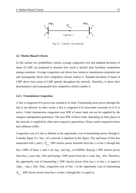
Fig. 4.1 – L<strong>in</strong>e No. i of a network<br />
In this section two probabilistic criteria, average congestion cost and standard deviation of<br />
mean of LMP, are proposed to measure how much a specific plan facilitates competition<br />
among customers. Average congestion cost shows how <strong>in</strong>tensive transmission constra<strong>in</strong>ts are<br />
and consequently shows how competitive electric market is. Standard deviation of mean of<br />
LMP shows how mean of LMP spreads throughout the network. Therefore, it shows how<br />
discrim<strong>in</strong>ative and consequently how competitive electric market is.<br />
4.2.1 <strong>Transmission</strong> Congestion<br />
A l<strong>in</strong>e is congested if its power has reached to its limit. Transmitt<strong>in</strong>g more power through this<br />
l<strong>in</strong>e is not allowed. In other words, a l<strong>in</strong>e is congested if its associated constra<strong>in</strong>t <strong>in</strong> (3.3) is<br />
active. Under transmission congestion next MW of some loads can not be supplied by the<br />
cheapest undispatched generation. The next MW of these loads, depend<strong>in</strong>g on their places <strong>in</strong><br />
the network, is supplied by other more expensive generations. Hence, under congestion buses<br />
have different LMPs.<br />
Congestion cost of a l<strong>in</strong>e is def<strong>in</strong>ed as the opportunity cost of transmitt<strong>in</strong>g power through it.<br />
Consider figure 4.1, l<strong>in</strong>e i of a network is depicted <strong>in</strong> this figure. The end buses of this l<strong>in</strong>e<br />
numerated with i1 and i2.<br />
Pl MW electric power transmits from bus i1 to bus i2 through this<br />
i i<br />
1 2<br />
l<strong>in</strong>e. LMPs of buses i1 and i2 are<br />
lmp i and<br />
1<br />
lmp i <strong>in</strong> $/MWhr. Buy<strong>in</strong>g 1 MW electric power<br />
2<br />
from bus i1 costs lmp i $/hr and buy<strong>in</strong>g 1 MW power from bus i2 costs 1<br />
i2<br />
lmp $/hr. Therefore,<br />
the opportunity cost of transmitt<strong>in</strong>g 1 MW electric power from bus i1 to bus i2 is equal to<br />
( i2<br />
i1<br />
lmp − lmp ) $/hr. Thus, congestion cost of l<strong>in</strong>e i or the opportunity cost of transmitt<strong>in</strong>g<br />
Pl MW electric power from bus i1 to bus i2 through l<strong>in</strong>e i is equal to:<br />
i i<br />
1 2<br />
lmp i<br />
lmp<br />
1<br />
i2<br />
i1<br />
Pl i i<br />
1 2<br />
L<strong>in</strong>e No. i<br />
i2