Transmission Expansion Planning in Deregulated Power ... - tuprints

4 Market Based Criteria 35
In the rest of this thesis “average congestion cost” is used instead of “average of total
congestion cost of the network”.
4.2.2 Flatness of Price Profile
Again consider a network with Nb buses and Nl lines. Suppose some plans were suggested for
transmission expansion. Assume PDFs of LMPs were computed for each plan using Nr
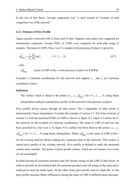
samples. The mean of LMP of bus i over Nr samples in the presence of plan k is given by:
k 1
k
µ lmp = lmpi,
j i=1, 2,…, Nb (4.7)
i N
Nr
∑
r j=
1
with:
k µ mean of LMP of bus i in the presence of plan k in $/MWhr
lmp
i
Consider a Cartesian coordination for the network and suppose x i , and y i are Cartesian
coordinates of bus i.
Definition:
The surface which is fitted to the points ( x i , y i , µ ) for i=1, 2,…, Nb using linear
k
lmpi
interpolation method is named piece profile of the network in the presence of plan k.
Price profile always passes through all data points. The z magnitude of other points is
determined by linear interpolation. Consider the example of section 3.3. The 8-bus network of
section 3.3 with the associated PDFs of LMPs is shown in figure 4.2. Figure 4.3 shows the 8bus
network on the xy-plane of Cartesian coordination. The mean of LMP of each bus has
been specified by a bar over it. In figure 4.4 a surface has been fitted to the points ( x i , y i ,
0
0
µ lmp ) for i=1, 2,…, 8 using linear interpolation. Where µ
i
lmp is the mean of LMP of bus i
i
for the existing network (before adding any expansion plan to the network). This surface is
named price profile of the existing network. Price profile is defined to make the presented
criteria more sensible. The points of price profile surface, which are not located over a bus,
are not meaningful.
In nodal pricing all customers purchase and sell electric energy at the LMP of their buses. In
order to provide an environment that all customers purchase and sell energy at the same price,
nodal prices must be made equal. On the other word, price profile must be made flat. As the
price profile becomes flatter, differences among the mean of LMP of different buses decrease.