Conference, Proceedings
Conference, Proceedings
Conference, Proceedings

Create successful ePaper yourself
Turn your PDF publications into a flip-book with our unique Google optimized e-Paper software.
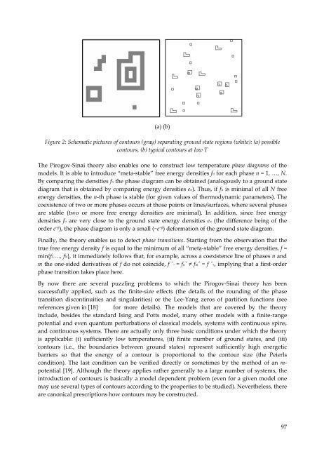
(a) (b)<br />
Figure 2: Schematic pictures of contours (gray) separating ground state regions (white): (a) possible<br />
contours, (b) typical contours at low T<br />
The Pirogov‐Sinai theory also enables one to construct low temperature phase diagrams of the<br />
models. It is able to introduce “meta‐stable” free energy densities fn for each phase n = 1, …, N.<br />
By comparing the densities fn the phase diagram can be obtained (analogously to a ground state<br />
diagram that is obtained by comparing energy densities en). Thus, if fn is minimal of all N free<br />
energy densities, the n‐th phase is stable (for given values of thermodynamic parameters). The<br />
coexistence of two or more phases occurs at those points or lines/surfaces, where several phases<br />
are stable (two or more free energy densities are minimal). In addition, since free energy<br />
densities fn are very close to the ground state energy densities en (the difference being of the<br />
order e −β ), the phase diagram is only a small (~e −β ) deformation of the ground state diagram.<br />
Finally, the theory enables us to detect phase transitions. Starting from the observation that the<br />
true free energy density f is equal to the minimum of all “meta‐stable” free energy densities, f =<br />
min{f1,…, fN}, it immediately follows that, for example, across a coexistence line of phases n and<br />
m the one‐sided derivatives of f do not coincide, f ′− = fn′ ≠ fm′ = f ′+, implying that a first‐order<br />
phase transition takes place here.<br />
By now there are several puzzling problems to which the Pirogov‐Sinai theory has been<br />
successfully applied, such as the finite‐size effects (the details of the rounding of the phase<br />
transition discontinuities and singularities) or the Lee‐Yang zeros of partition functions (see<br />
references given in [18] for more details). The models that are covered by the theory<br />
include, besides the standard Ising and Potts model, many other models with a finite‐range<br />
potential and even quantum perturbations of classical models, systems with continuous spins,<br />
and continuous systems. There are actually only three basic conditions under which the theory<br />
is applicable: (i) sufficiently low temperatures, (ii) finite number of ground states, and (iii)<br />
contours (i.e., the boundaries between ground states) represent sufficiently high energetic<br />
barriers so that the energy of a contour is proportional to the contour size (the Peierls<br />
condition). The last condition can be verified directly or sometimes by the method of an m‐<br />
potential [19]. Although the theory applies rather generally to a large number of systems, the<br />
introduction of contours is basically a model dependent problem (even for a given model one<br />
may use several types of contours according to the properties to be studied). Nevertheless, there<br />
are canonical prescriptions how contours may be constructed.<br />
97