RiskMetrics™ —Technical Document

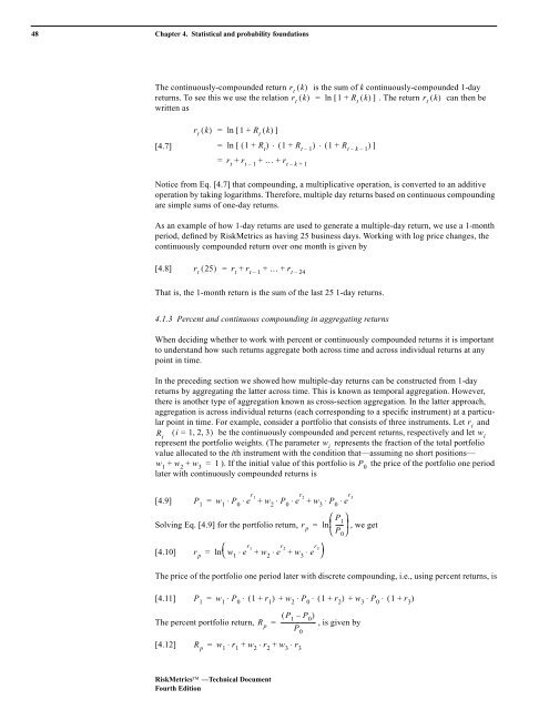
48 Chapter 4. Statistical and probability foundations
The continuously-compounded return r t
( k)
is the sum of k continuously-compounded 1-day
returns. To see this we use the relation r t
( k) = ln [ 1+
R t
( k)
] . The return r t
( k)
can then be
written as
[4.7]
r t
( k) = ln [ 1+
R t
( k)
]
= ln [ ( 1 + R t
) ⋅ ( 1+
R ) 1 R t – 1
⋅ ( + t – k –
)]
1
= r t
+ r t – 1
+ … + r t k
– + 1
Notice from Eq. [4.7] that compounding, a multiplicative operation, is converted to an additive
operation by taking logarithms. Therefore, multiple day returns based on continuous compounding
are simple sums of one-day returns.
As an example of how 1-day returns are used to generate a multiple-day return, we use a 1-month
period, defined by RiskMetrics as having 25 business days. Working with log price changes, the
continuously compounded return over one month is given by
[4.8]
r t
( 25) = r t
+ r t – 1
+ … + r t – 24
That is, the 1-month return is the sum of the last 25 1-day returns.
4.1.3 Percent and continuous compounding in aggregating returns
When deciding whether to work with percent or continuously compounded returns it is important
to understand how such returns aggregate both across time and across individual returns at any
point in time.
In the preceding section we showed how multiple-day returns can be constructed from 1-day
returns by aggregating the latter across time. This is known as temporal aggregation. However,
there is another type of aggregation known as cross-section aggregation. In the latter approach,
aggregation is across individual returns (each corresponding to a specific instrument) at a particular
point in time. For example, consider a portfolio that consists of three instruments. Let r i
and
R i
( i = 123 , , ) be the continuously compounded and percent returns, respectively and let w i
represent the portfolio weights. (The parameter w i
represents the fraction of the total portfolio
value allocated to the ith instrument with the condition that—assuming no short positions—
w 1
+ w 2
+ w 3
= 1). If the initial value of this portfolio is P 0
the price of the portfolio one period
later with continuously compounded returns is
[4.9] P 1
w 1
P 0
e r 1
⋅ ⋅ w 2
P 0
e r 2
⋅ ⋅ w 3
P 0
e r 3
=
+ + ⋅ ⋅
⎛P 1
⎞
Solving Eq. [4.9] for the portfolio return, r p
= ln⎜-----
⎟ , we get
⎝ ⎠
⎛
[4.10] r p
w 1
e r 1
⋅ w 2
e r 2
⋅ w 3
e r 3⎞
= ln⎝
+ + ⋅ ⎠
The price of the portfolio one period later with discrete compounding, i.e., using percent returns, is
P 0
[4.11]
P 1
= w 1
⋅ P 0
⋅ ( 1 + r 1
) + w 2
⋅ P 0
⋅ ( 1+
r 2
) + w 3
⋅ P 0
⋅ ( 1+
r 3
)
( P
The percent portfolio return, R 1
– P 0
)
p
= ------------------------ , is given by
P 0
[4.12]
R p
= w 1
⋅ r 1
+ w 2
⋅ r 2
+ w 3
⋅ r 3
RiskMetrics —Technical Document
Fourth Edition