RiskMetrics™ —Technical Document

72 Chapter 4. Statistical and probability foundations
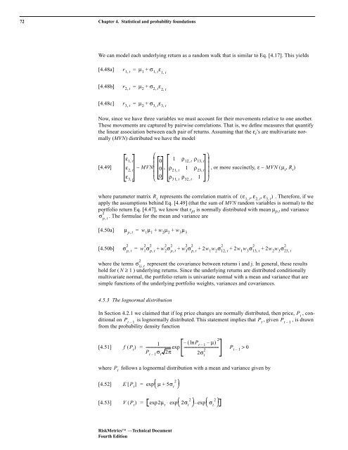
We can model each underlying return as a random walk that is similar to Eq. [4.17]. This yields
[4.48a]
[4.48b]
[4.48c]
,
= µ 1
+ σ 1 t
r 1 t
r 2 t
,
= µ 2
+ σ 2 t
r 3 t
,
= µ 2
+ σ 3 t
,
ε 1,
t
,
ε 2,
t
,
ε 3,
t
Now, since we have three variables we must account for their movements relative to one another.
These movements are captured by pairwise correlations. That is, we define measures that quantify
the linear association between each pair of returns. Assuming that the ε t ’s are multivariate normally
(MVN) distributed we have the model
⎛
⎞
ε 1,
t ⎜ 0
1 ρ 12, t
ρ 13,
t ⎟
[4.49] ε 2,
t
∼ MVN
⎜
0 ,
⎟
⎜ ρ 21, t
1 ρ 23,
t ⎟ , or more succinctly, ε∼
MVN ( µ t
, R t
)
⎜
ε 3, t ⎝
0
⎟
ρ 31, t
ρ 32, t
1 ⎠
where parameter matrix R t
represents the correlation matrix of ( ε 1, t
, ε 2, t
, ε 3,
t
) . Therefore, if we
apply the assumptions behind Eq. [4.49] (that the sum of MVN random variables is normal) to the
portfolio return Eq. [4.47], we know that r pt is normally distributed with mean µ p,t and variance
2
. The formulae for the mean and variance are
σ pt ,
[4.50a]
µ pt
,
= w 1
µ 1
+ w 2
µ 2
+ w 3
µ 3
[4.50b]
2
σ pt ,
=
2 2
w 1σpt
,
2 2
w 2σpt
,
2 2
w 3σpt
,
+ + + 2w 1
w 2
σ 12,
t
+ 2w 1
w 3
σ 13,
t
+
2
2
2
2w 2
w 3
σ 23,
t
2
σ ij t
where the terms ,
represent the covariance between returns i and j. In general, these results
hold for ( N ≥ 1 ) underlying returns. Since the underlying returns are distributed conditionally
multivariate normal, the portfolio return is univariate normal with a mean and variance that are
simple functions of the underlying portfolio weights, variances and covariances.
4.5.3 The lognormal distribution
In Section 4.2.1 we claimed that if log price changes are normally distributed, then price, , conditional
on P t – 1
is lognormally distributed. This statement implies that P t
, given P t – 1
, is drawn
from the probability density function
P t
[4.51]
f
( P t
)
=
1 –( lnP ---------------------------
t – 1
– µ ) 2
exp -------------------------------------- P
2
t 1
>
P t – 1
σ t
2π 2σ t
–
0
where
[4.52]
[4.53]
P t
follows a lognormal distribution with a mean and variance given by
E[ P t
] =
⎛ 2⎞
exp⎝µ + 5σ t ⎠
V ( P t
) =
⎛ 2⎞
⎛ 2⎞
exp2µ t
⋅ exp⎝2σ t ⎠–exp⎝σ t ⎠
RiskMetrics —Technical Document
Fourth Edition