RiskMetrics™ —Technical Document

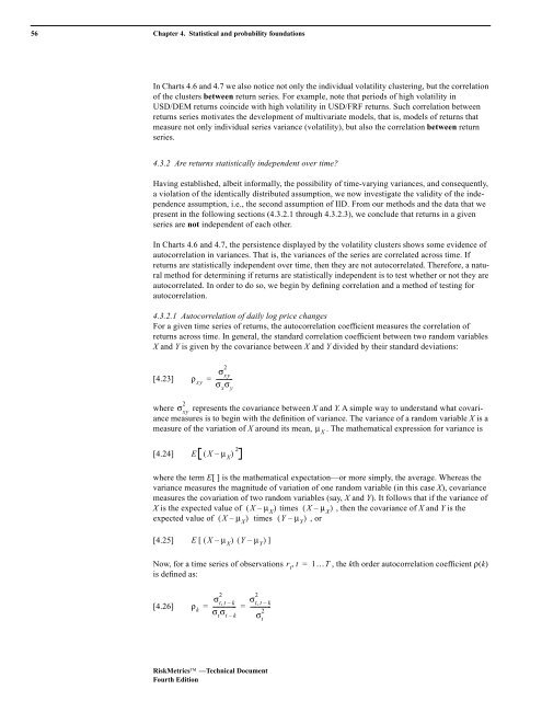
56 Chapter 4. Statistical and probability foundations
In Charts 4.6 and 4.7 we also notice not only the individual volatility clustering, but the correlation
of the clusters between return series. For example, note that periods of high volatility in
USD/DEM returns coincide with high volatility in USD/FRF returns. Such correlation between
returns series motivates the development of multivariate models, that is, models of returns that
measure not only individual series variance (volatility), but also the correlation between return
series.
4.3.2 Are returns statistically independent over time?
Having established, albeit informally, the possibility of time-varying variances, and consequently,
a violation of the identically distributed assumption, we now investigate the validity of the independence
assumption, i.e., the second assumption of IID. From our methods and the data that we
present in the following sections (4.3.2.1 through 4.3.2.3), we conclude that returns in a given
series are not independent of each other.
In Charts 4.6 and 4.7, the persistence displayed by the volatility clusters shows some evidence of
autocorrelation in variances. That is, the variances of the series are correlated across time. If
returns are statistically independent over time, then they are not autocorrelated. Therefore, a natural
method for determining if returns are statistically independent is to test whether or not they are
autocorrelated. In order to do so, we begin by defining correlation and a method of testing for
autocorrelation.
4.3.2.1 Autocorrelation of daily log price changes
For a given time series of returns, the autocorrelation coefficient measures the correlation of
returns across time. In general, the standard correlation coefficient between two random variables
X and Y is given by the covariance between X and Y divided by their standard deviations:
[4.23]
ρ xy
=
2
σ xy
-----------
σ x
σ y
2
σ xy
where represents the covariance between X and Y. A simple way to understand what covariance
measures is to begin with the definition of variance. The variance of a random variable X is a
measure of the variation of X around its mean, . The mathematical expression for variance is
µ X
[4.24]
E ( X – µ X
) 2
where the term E[ ] is the mathematical expectation—or more simply, the average. Whereas the
variance measures the magnitude of variation of one random variable (in this case X), covariance
measures the covariation of two random variables (say, X and Y). It follows that if the variance of
X is the expected value of ( X – µ X
) times ( X – µ X
) , then the covariance of X and Y is the
expected value of ( X – µ X
) times ( Y – µ Y
) , or
[4.25]
E[ ( X – µ X
) ( Y – µ Y
)]
Now, for a time series of observations r t
, t = 1…T , the kth order autocorrelation coefficient ρ(k)
is defined as:
[4.26]
2
,
2
σ t t
2
σ t
σ
ρ t t – k
k
= ---------------- = -------------- , – k
σ t
σ t – k
RiskMetrics —Technical Document
Fourth Edition