RiskMetrics™ —Technical Document

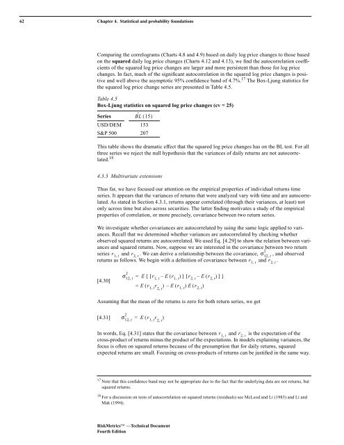
62 Chapter 4. Statistical and probability foundations
Comparing the correlograms (Charts 4.8 and 4.9) based on daily log price changes to those based
on the squared daily log price changes (Charts 4.12 and 4.13), we find the autocorrelation coefficients
of the squared log price changes are larger and more persistent than those for log price
changes. In fact, much of the significant autocorrelation in the squared log price changes is positive
and well above the asymptotic 95% confidence band of 4.7%. 17 The Box-Ljung statistics for
the squared log price change series are presented in Table 4.5.
Table 4.5
Box-Ljung statistics on squared log price changes (cv = 25)
Series BL ˆ ( 15)
USD/DEM 153
S&P 500 207
This table shows the dramatic effect that the squared log price changes has on the BL test. For all
three series we reject the null hypothesis that the variances of daily returns are not autocorrelated.
18
4.3.3 Multivariate extensions
Thus far, we have focused our attention on the empirical properties of individual returns time
series. It appears that the variances of returns that were analyzed vary with time and are autocorrelated.
As stated in Section 4.3.1, returns appear correlated (through their variances, at least) not
only across time but also across securities. The latter finding motivates a study of the empirical
properties of correlation, or more precisely, covariance between two return series.
We investigate whether covariances are autocorrelated by using the same logic applied to variances.
Recall that we determined whether variances are autocorrelated by checking whether
observed squared returns are autocorrelated. We used Eq. [4.29] to show the relation between variances
and squared returns. Now, suppose we are interested in the covariance between two return
2
series r 1, t
and r 2, t
. We can derive a relationship between the covariance, σ 12,
t
, and observed
returns as follows. We begin with a definition of covariance between and .
r 1, t
r 2,
t
[4.30]
2
σ 12,
t
= E{ [ r 1, t
– E( r 1,
t
)] [ r 2, t
– E( r 2,
t
)]}
= E ( r ) E r 1 t
– ( 1 ,
)E( r t 2,
t
)
,
r 2,
t
Assuming that the mean of the returns is zero for both return series, we get
[4.31]
2
σ 12,
t
=
E ( r ) 1 t
,
r 2,
t
In words, Eq. [4.31] states that the covariance between ,
and r 2,
t
is the expectation of the
cross-product of returns minus the product of the expectations. In models explaining variances, the
focus is often on squared returns because of the presumption that for daily returns, squared
expected returns are small. Focusing on cross-products of returns can be justified in the same way.
r 1 t
17 Note that this confidence band may not be appropriate due to the fact that the underlying data are not returns, but
squared returns.
18 For a discussion on tests of autocorrelation on squared returns (residuals) see McLeod and Li (1983) and Li and
Mak (1994).
RiskMetrics —Technical Document
Fourth Edition