RiskMetrics⢠âTechnical Document
RiskMetrics⢠âTechnical Document
RiskMetrics⢠âTechnical Document

Create successful ePaper yourself
Turn your PDF publications into a flip-book with our unique Google optimized e-Paper software.
58 Chapter 4. Statistical and probability foundations<br />
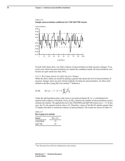
Chart 4.9<br />
Sample autocorrelation coefficients for USD S&P 500 returns<br />
Autocorrelation<br />
0.08<br />
0.06<br />
0.04<br />
0.02<br />
0<br />
-0.02<br />
-0.04<br />
-0.06<br />
-0.08<br />
-0.10<br />
1 12 23 34 45 56 67 78 89 100<br />
Lag (days)<br />
Overall, both charts show very little evidence of autocorrelation in daily log price changes. Even<br />
in the cases where the autocorrelations are outside the confidence bands, the autocorrelation coefficients<br />
are quite small (less than 10%).<br />
4.3.2.2 Box-Ljung statistic for daily log price changes<br />
While the above charts are useful for getting a general idea about the level of autocorrelation of<br />
log price changes, there are more formal methods of testing for autocorrelation. An often cited<br />
method is the Box-Ljung (BL) test statistic, 14 defined as<br />
[4.28]<br />
BL ( p) = T ⋅ ( T + 2)<br />
p<br />
∑<br />
k = 1<br />
ρ k<br />
2<br />
-----------<br />
T – k<br />
Under the null hypothesis that a time series is not autocorrelated, BL ( p ), is distributed chisquared<br />
with p degrees of freedom. In Eq. [4.28], p denotes the number of autocorrelations used to<br />
estimate the statistic. We applied this test to the USD/DEM and S&P 500 returns for p = 15. In this<br />
case, the 5% chi-squared critical value is 25. Therefore, values of the BL(10) statistic greater than<br />
25 implies that there is statistical evidence of autocorrelation. The results are shown in Table 4.3.<br />
Table 4.3<br />
Box-Ljung test statistic<br />
Series<br />
BL ˆ ( 15)<br />
USD/DEM 15<br />
S&P 500 25<br />
14 See West and Cho (1995) for modifications to this statistic.<br />
RiskMetrics —Technical <strong>Document</strong><br />
Fourth Edition