RiskMetrics™ —Technical Document

78 Chapter 5. Estimation and forecast
Academic research has compared the forecasting ability of implied and historical volatility models.
The evidence of the superior forecasting ability of historical volatility over implied volatility
is mixed, depending on the time series considered. For example, Xu and Taylor (1995, p. 804) note
that, “prior research concludes that volatility predictors calculated from options prices are better
predictors of future volatility than standard deviations calculated from historical asset price data.”
Kroner, Kneafsey and Claessens (1995, p. 9), on the other hand, note that researchers are beginning
to conclude that GARCH (historical based) forecasts outperform implied volatility forecasts.
Since implied standard deviation captures market expectations and pure time series models rely
solely on past information, these models can be combined to forecast the standard deviation of
returns.
5.2 RiskMetrics forecasting methodology
RiskMetrics uses the exponentially weighted moving average model (EWMA) to forecast variances
and covariances (volatilities and correlations) of the multivariate normal distribution. This
approach is just as simple, yet an improvement over the traditional volatility forecasting method
that relies on moving averages with fixed, equal weights. This latter method is referred to as the
simple moving average (SMA) model.
5.2.1 Volatility estimation and forecasting 1
One way to capture the dynamic features of volatility is to use an exponential moving average of
historical observations where the latest observations carry the highest weight in the volatility estimate.
This approach has two important advantages over the equally weighted model. First, volatility
reacts faster to shocks in the market as recent data carry more weight than data in the distant
past. Second, following a shock (a large return), the volatility declines exponentially as the weight
of the shock observation falls. In contrast, the use of a simple moving average leads to relatively
abrupt changes in the standard deviation once the shock falls out of the measurement sample,
which, in most cases, can be several months after it occurs.
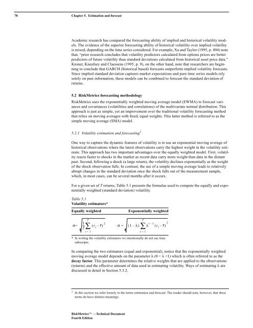
For a given set of T returns, Table 5.1 presents the formulae used to compute the equally and exponentially
weighted (standard deviation) volatility.
Table 5.1
Volatility estimators*
Equally weighted
Exponentially weighted
T
∑
1
σ= -- ( r
T t
– r ) 2
σ = ( 1 – λ) λ t – 1
( r t
– r) 2
t = 1
* In writing the volatility estimators we intentionally do not use time
subscripts.
T
∑
t = 1
In comparing the two estimators (equal and exponential), notice that the exponentially weighted
moving average model depends on the parameter λ (0 < λ