RiskMetrics™ —Technical Document

50 Chapter 4. Statistical and probability foundations
4.2.1 Random walk model for single-price assets
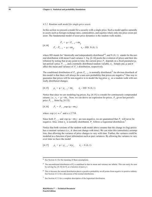
In this section we present a model for a security with a single price. Such a model applies naturally
to assets such as foreign exchange rates, commodities, and equities where only one price exists per
asset. The fundamental model of asset price dynamics is the random walk model,
[4.14]
P t
= µ + P t – 1
+ σε t
P t
– P t – 1
= µ + σε ,
t
ε t
∼IID N ( 0,
1)
where IID stands for “identically and independently distributed” 4 , and N ( 01 , ) stands for the normal
distribution with mean 0 and variance 1. Eq. [4.14] posits the evolution of prices and their distribution
by noting that at any point in time, the current price P t
depends on a fixed parameter µ,
last period’s price P t – 1
, and a normally distributed random variable, ε t
. Simply put, µ and σ
affect the mean and variance of ’s distribution, respectively.
P t
The conditional distribution of P , given , is normally distributed. 5 t
P t – 1
An obvious drawback of
this model is that there will always be a non-zero probability that prices are negative. 6 One way to
guarantee that prices will be non-negative is to model the log price p t
as a random walk with normally
distributed changes.
[4.15]
p t
= µ + p t – 1
+ σε t
ε t
∼IID N ( 0,
1)
Notice that since we are modeling log prices, Eq. [4.15] is a model for continuously compounded
returns, i.e., r t
= µ + σε t
. Now, we can derive an expression for prices, P t
given last period’s
price from Eq. [4.15]:
P t 1
–
P t
P t 1
[4.16]
=
–
exp ( µ + σε t
)
where exp ( x)
≡ and e ≅ 2.718.
P t 1
e x
Since both –
and exp ( µ + σε t
) are non-negative, we are guaranteed that P t
will never be
negative. Also, when is normally distributed, follows a lognormal distribution. 7
ε t
Notice that both versions of the random walk model above assume that the change in (log) prices
has a constant variance (i.e., σ does not change with time). We can relax this (unrealistic) assumption,
thus allowing the variance of price changes to vary with time. Further, the variance could be
modeled as a function of past information such as past variances. By allowing the variance to vary
over time we have the model
P t
[4.17]
p t
= µ + p t – 1
+ σ t
ε t
ε t
∼ N ( 01 , )
4 See Section 4.3 for the meaning of these assumptions.
5 The unconditional distribution of P t is undefined in that its mean and variance are infinite. This can easily be seen
by solving Eq. [4.14] for P t as a function of past ε t ’s.
6 This is because the normal distribution places a positive probability on all points from negative to positive infinity.
See Section 4.5.2 for a discussion of the normal distribution.
7 See Section 4.5.3 for a complete description of the lognormal distribution.
RiskMetrics —Technical Document
Fourth Edition