RiskMetrics™ —Technical Document

66 Chapter 4. Statistical and probability foundations
The second class of models, the conditional distribution of returns, arises from evidence that
refutes the identically and independently distributed assumptions (as presented in Sections 4.3.1
and 4.3.2). Models in this category, such as the GARCH and Stochastic Volatility, treat volatility
as a time-dependent, persistent process. These models are important because they account for volatility
clustering, a frequently observed phenomenon among return series.
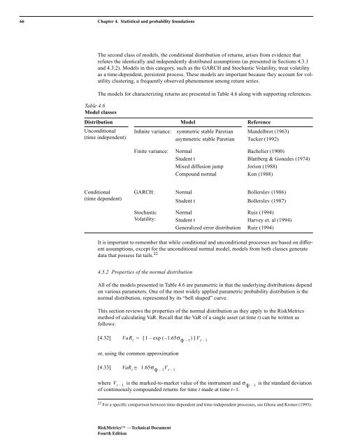
The models for characterizing returns are presented in Table 4.6 along with supporting references.
Table 4.6
Model classes
Distribution Model Reference
Unconditional
(time independent)
Infinite variance: symmetric stable Paretian Mandelbrot (1963)
asymmetric stable Paretian Tucker (1992)
Finite variance: Normal Bachelier (1900)
Student t Blattberg & Gonedes (1974)
Mixed diffusion jump Jorion (1988)
Compound normal Kon (1988)
Conditional
(time dependent)
GARCH: Normal Bollerslev (1986)
Student t Bollerslev (1987)
Stochastic
Volatility:
Normal Ruiz (1994)
Student t Harvey et. al (1994)
Generalized error distribution Ruiz (1994)
It is important to remember that while conditional and unconditional processes are based on different
assumptions, except for the unconditional normal model, models from both classes generate
data that possess fat tails. 22
4.5.2 Properties of the normal distribution
All of the models presented in Table 4.6 are parametric in that the underlying distributions depend
on various parameters. One of the most widely applied parametric probability distribution is the
normal distribution, represented by its “bell shaped” curve.
This section reviews the properties of the normal distribution as they apply to the RiskMetrics
method of calculating VaR. Recall that the VaR of a single asset (at time t) can be written as
follows:
[4.32]
VaR t
= [ 1 – exp (–
1.65σ tt–
1
)]V t – 1
or, using the common approximation
[4.33]
VaR t
≅ 1.65σ tt 1
–
V t–
1
V t 1
where –
is the marked-to-market value of the instrument and σ tt–
1
is the standard deviation
of continuously compounded returns for time t made at time t−1.
22 For a specific comparison between time-dependent and time-independent processes, see Ghose and Kroner (1993).
RiskMetrics —Technical Document
Fourth Edition