Spin-orbit coupling and electron-phonon scattering - Fachbereich ...
Spin-orbit coupling and electron-phonon scattering - Fachbereich ...
Spin-orbit coupling and electron-phonon scattering - Fachbereich ...

Create successful ePaper yourself
Turn your PDF publications into a flip-book with our unique Google optimized e-Paper software.
3.1 <strong>Spin</strong>-<strong>orbit</strong> driven coherent oscillations in a few-<strong>electron</strong> quantum dot 53<br />
2<br />
(a)<br />
-0.5 δ = 0 0.5<br />
(b)<br />
0.36<br />
1.5<br />
∆<br />
0<br />
E<br />
E<br />
1<br />
0.5<br />
0<br />
0 0.5 1 1.5<br />
B/B 0<br />
(c)<br />
2.0<br />
1.5<br />
0.8<br />
0.3<br />
1 2 3<br />
E<br />
0.24<br />
0.2<br />
∆<br />
0.1<br />
Figure 3.1: Spectral features of Rashba–coupled quantum dot as function of magnetic<br />
field. The parameters used are typical of InGaAs: g = −4, m/m e = 0.05<br />
with dot size l 0 = 150nm. Resonance occurs at B 0 = 90mT. (a) Low-lying<br />
excitation spectrum for spin-<strong>orbit</strong> <strong>coupling</strong> α = 0.8 × 10 −12 eVm. (b) Lowest<br />
lying anticrossing. Thick line is JC model showing anticrossing width ∆ 0 at<br />
δ = 0, <strong>and</strong> thin line is exact numerical result. (c) Plot of width ∆ n against central<br />
energy of anticrossing with the dot on resonance for different α in the range<br />
0.3−2.0×10 −12 eVm. The exact numerical results (circles) show excellent agreement<br />
with the square-root behaviour predicted by the JC model in this α range.<br />
with λ = l 2 0 γ −/2˜l l SO . This is the well-known Jaynes-Cummings model (JCM) of<br />
quantum optics. It is completely integrable, <strong>and</strong> has ground state |0,↓〉 with energy<br />
= (n + 1/2)ω − ± ∆ n /2 with<br />
E G = −E z /2 independent of <strong>coupling</strong>. The rest of the JCM Hilbert space decomposes<br />
into two-dimensional subspaces {|n,↑〉,|n + 1,↓〉; n = 0,1,...}. Diagonalisation<br />
in each subspace gives the energies E α<br />
(n,±)<br />
detuning δ ≡ ω − − E z <strong>and</strong> ∆ n ≡ √ δ 2 + 4λ 2 (n + 1). The eigenstates are<br />
|ψ (n,±)<br />
α<br />
〉 = cosθ (n,±) |n,↑〉 + sinθ α (n,±) |n + 1,↓〉, (3.7)<br />
α<br />
with tanθ (n,±)<br />
α = (δ ± ∆ n )/2λ(n + 1) 1/2 .<br />
Figure 3.1a shows a portion of the excitation spectrum obtained by exact numerical<br />
diagonalisation for a typical dot in InGaAs. The approximate H JC de-