Spin-orbit coupling and electron-phonon scattering - Fachbereich ...

More documents

Recommendations

Info

54 Rashba spin-orbit coupling in quantum dots scribes the energy levels of the system to within 10% of the typical anticrossing width and 1% of ω 0 . This small discrepancy is visible in Fig. 3.1b. In the following, we are only concerned with the lowest-lying energy states in the dots. Without SO interaction, these states are described by n + = 0 – indicating that the states converge to the lowest Landau level in the high-field limit, and by n − corresponding to the quantum number of angular momentum. The SO interaction thus couples two states of adjacent angular momentum and opposite spin. The detuning δ uniquely identifies ω c for fixed material parameters and dot size. Under the assumptions of the constant interaction model [108], the most important prediction of this model for linear transport is that, with the dot on resonance, the addition-energy spectrum for the first few electrons (up to 18 here) is described by a sequence of well-separated anticrossings, the width of which increases as α √ n + 1. This behaviour is shown in Fig. 3.1c, and its observation would be confirmation of our JC model, and would permit a determination of α in quantum dots. We now describe the procedure for observing spin-orbit driven Rabi oscillations. Our proposal is somewhat similar to that of Nakamura [6] with a voltage pulse driving the system, but with the crucial difference that the oscillations here are induced, not by a change in the detuning, but by a change in the SO coupling strength. We operate in the non-linear transport regime and address a single two-level system by being near resonance and by tuning the chemical potentials of the leads close to the n-th anticrossing. The SO coupling is set to α 1 and the states taking part in the oscillation are eigenstates of H JC (α 1 ), namely ψ ± α 1 , which are situated symmetrically around the chemical potential of the right lead µ R , see Fig. 3.2a. The temperature is taken smaller than the detuning k B T ≪ δ to avoid the effects of thermal broadening. Assuming Coulomb blockade and considering first-order sequential tunnelling only, electrons can either tunnel from the left lead into the dot via state ψ + α 1 and subsequently leave to the right or, alternatively, tunnel to state ψ − α 1 blockading the dot, see Fig. 3.2b. Assuming tunnelling through the left/right barrier at a constant rate Γ L/R , we set Γ L > Γ R to assure that the dot is preferentially filled from the left; thus maximising the current. On average then, the dot will be initialised in state ψ − α 1 for times t i > Γ −1 R . Having trapped an electron in this state, we apply a voltage pulse to the gate. This has two effects. Firstly, this change in voltage alters the SO coupling to a new value α 2 . Since this change is performed non-adiabatically, the electron remains in the initial eigenstate ψ − α 1 until Rabi oscillations begin between this state and ψ + α 1 under the influence of the new Hamiltonian H JC (α 2 ). Secondly, the TLS is drawn below both chemical potentials, assuring that oscillations can occur without tunnelling out of the dot, see Fig. 3.2c. After a time t p , the gate voltage is returned to its initial value, and the TLS resumes both to its original position and coupling α 1 , as in Fig. 3.2d. Tunnelling
£££££££££££££¢¢¢¢¢¢¢¢¢¢¢¢¢ ¡¡¡¡¡¡¡¡¡¡¡¡¡¡ ¥¥¥¥¥¥¥¥¥¥¥¥¥¤¤¤¤¤¤¤¤¤¤¤¤¤ 3.1 Spin-orbit driven coherent oscillations in a few-electron quantum dot 55 PSfrag replacements (a) § § ¨§¨ ¦§¦ ¨§¨ ¦§¦ § § (b) ψ + α 1 µ L µ R Γ L Γ R ¨§¨ ¦§¦ ψ − α 1 ¨§¨ ¦§¦ § § § § ¨§¨ ¦§¦ ¨§¨ ¦§¦ § § ¨§¨ ¦§¦ ¨§¨ ¦§¦ ¨§¨ ¦§¦ ¨§¨ ¦§¦ ¨§¨ ¦§¦ ¨§¨ ¦§¦ ¨§¨ ¦§¦ § § § § (c) α 1 α 1 § § (d) § § § § § § § § § ©§© § § § ©§© § § § ©§© § § α 2 § § § § § Γ 2 § § § Γ 1 α 1 ©§© § ©§© § § § ©§© § § § ©§© § § § ©§© 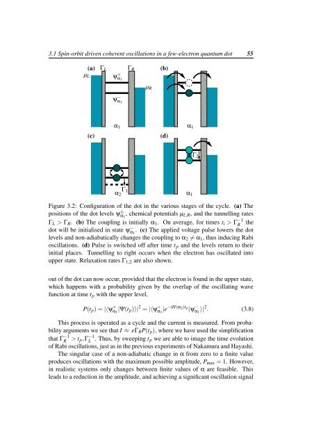Figure 3.2: Configuration of the dot in the various stages of the cycle. (a) The positions of the dot levels ψ ± α 1 , chemical potentials µ L,R , and the tunnelling rates Γ L > Γ R . (b) The coupling is initially α 1 . On average, for times t i > Γ −1 R the dot will be initialised in state ψ − α 1 . (c) The applied voltage pulse lowers the dot levels and non-adiabatically changes the coupling to α 2 ≠ α 1 , thus inducing Rabi oscillations. (d) Pulse is switched off after time t p and the levels return to their initial places. Tunnelling to right occurs when the electron has oscillated into upper state. Relaxation rates Γ 1,2 are also shown. out of the dot can now occur, provided that the electron is found in the upper state, which happens with a probability given by the overlap of the oscillating wave function at time t p with the upper level, P(t p ) = |〈ψ + α 1 |Ψ(t p )〉| 2 = |〈ψ + α 1 |e −iH(α 2)t p |ψ − α 1 〉| 2 . (3.8) This process is operated as a cycle and the current is measured. From probability arguments we see that I ≈ eΓ R P(t p ), where we have used the simplification that Γ −1 R > t p,Γ −1 L . Thus, by sweeping t p we are able to image the time evolution of Rabi oscillations, just as in the previous experiments of Nakamura and Hayashi. The singular case of a non-adiabatic change in α from zero to a finite value produces oscillations with the maximum possible amplitude, P max = 1. However, in realistic systems only changes between finite values of α are feasible. This leads to a reduction in the amplitude, and achieving a significant oscillation signal
Page 1 and 2:
Interaction and confinement in nano
Page 3 and 4:
Abstract iii Abstract It is the pur
Page 5:
Publications v Publications Some of
Page 8 and 9:
2 Table of Contents 3 Rashba spin-o
Page 10 and 11: 4 Introduction (phonons). Therefore
Page 12 and 13: 6 Introduction Figure 1: Scanning e
Page 15 and 16: Chapter 1 The Rashba effect Effects
Page 17 and 18: 1.2 The model 11 the position-depen
Page 19 and 20: 1.3 Rashba effect in a perpendicula
Page 21 and 22: Chapter 2 Rashba spin-orbit couplin
Page 23 and 24: 2.1 Rashba effect and magnetic fiel
Page 31 and 32: PSfrag replacements 2.1 Rashba effe
Page 33 and 34: 2.2 Spectral properties, various li
Page 39 and 40: 2.3 Electron transport in one-dimen
Page 41 and 42: PSfrag replacements 2.3 Electron tr
Page 47 and 48: PSfrag replacements 2.3 Electron tr
Page 51 and 52: 2.4 Summary 45 For weak SO coupling
Page 53 and 54: 2.4 Summary 47 splitting can become
Page 55 and 56: Chapter 3 Rashba spin-orbit couplin
Page 57 and 58: 3.1 Spin-orbit driven coherent osci
Page 59: 3.1 Spin-orbit driven coherent osci
Page 63 and 64: 0 0.5 1.5 3.1 Spin-orbit driven coh
Page 65 and 66: 3.2 Introduction to quantum dots an
Page 75 and 76: PSfrag replacements 3.2 Introductio
Page 77 and 78: 3.3 Effects of relaxation 71 page 5
Page 79 and 80: 3.3 Effects of relaxation 73 The re
Page 81 and 82: 3.3 Effects of relaxation 75 with q
Page 83 and 84: 3.3 Effects of relaxation 77 eh 14
Page 85 and 86: Chapter 4 Conclusion In this part o
Page 87 and 88: Tuneable quantum dots connected to
Page 89: Part II Phonon confinement in nanos
Page 92 and 93: 86 Introduction to electron-phonon
Page 94 and 95: 88 Introduction to electron-phonon
Page 96 and 97: 90 Coupled quantum dots in a phonon
Page 102 and 103: ) ) ) ) 3 4 + ) * - 96 Coupled quan
Page 106 and 107: 100 Coupled quantum dots in a phono
Page 108 and 109: 102 Coupled quantum dots in a phono
Page 110 and 111:
PSfrag replacements 1042 Coupled qu
Page 112 and 113:
106 Coupled quantum dots in a phono
Page 114 and 115:
108 Coupled quantum dots in a phono
Page 116 and 117:
110 Conclusion due to phonon van-Ho
Page 119 and 120:
Appendix A Jaynes-Cummings model Th
Page 121 and 122:
Appendix B Fock-Darwin representati
Page 123 and 124:
Appendix C Evaluation of the phonon
Page 125 and 126:
Appendix D Matrix elements of dot e
Page 127 and 128:
121 with λ ± l (q ‖) = F n B pz
Page 129 and 130:
Bibliography [1] G. Bergmann, Phys.
Page 131 and 132:
Bibliography 125 [31] M. Pletyukhov
Page 133 and 134:
Bibliography 127 [72] T. Schäpers,
Page 135 and 136:
Bibliography 129 [109] U. Merkt, J.
Page 137 and 138:
Bibliography 131 [144] B. Auld, Aco
Page 139 and 140:
Bibliography 133 [182] A. A. Kisele
Page 141:
Acknowledgements Finally, I would l
show all

Spin-orbit coupling and electron-phonon scattering - Fachbereich ...

You also want an ePaper? Increase the reach of your titles

Delete template?

Save as template?