CRC Report No. A-34 - Coordinating Research Council

April 2005
the DRI data was consistent with variability in inter-laboratory blind comparisons (Apel et al.,
1999). The simulated ambient samples from the CAMx simulations were post-processed by
adding random sampling noise to obtain a target level of variability for each species. The
sampling noise sometimes resulted in negative concentrations that were then treated as missing
data.
We analyzed ambient data obtained by DRI in an October 1995 Los Angeles study that has been
used in previous CRC projects (Fujita et. al., 1997a). The analysis focused on morning samples
when variability should be most related to source variability and measurement artifacts and least
related to different chemical aging. The October 1995 data set included 24 VOC canister
samples that were collected at eight sites across the Los Angeles urban area from 6 to 7 am or 7
to 8 am on October 10-12, 1995 (Fujita et al., 1997). The sites included Azusa, Burbank,
Lynwood, Long Beach, Los Angeles North Main and Pico Rivera. The VOC data were
classified into PAMS and other species, and sum of the PAMS species compared to the total
NMHC (TNMHC) in Figure 2-2. For most samples the PAMS species accounted for about 70%
of TNHMC except for two samples from Pico Rivera that were excluded from further analysis.
The weight fraction of the PAMS species (i.e., relative to the sum of PAMS species) was
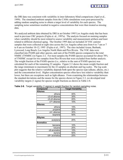
calculated for each of the remaining 22 samples. Figure 2-3 shows the mean weight fraction and
the range (minimum to maximum) for the 22 samples on absolute and log scales. The log scale
plot suggests that the relative variability depends both upon the species type (alkane, alkene, etc.)
and the concentration level. Higher concentration species often have less relative variability than
lower, but there are exceptions such as light alkanes. From examining the relationships between
the standard deviations and the means for the species shown in Figure 2-3, we developed total
variability targets (1 sigma) for species weight fractions as shown in Table 2-8.
Table 2-8. Target variability (1 sigma) in weight fraction for random sampling noise.
Compound
Target Variability
Alkanes
ethane 40%
c3-c4 alkanes 35%
c5-c6 alkanes 20%
c7+ alkanes 10%
Alkenes
ethene 15%
propene 20%
c4+ alkenes 30%
isoprene 50%
Alkynes
acetylene 20%
Aromatics
benzene 10%
toluene 20%
c8 aromatics 15%
styrene 50%
c9+ aromatics 25%
H:\crca34-receptor\report\Final\sec2.doc 2-11