PHD Thesis - Institute for Computer Graphics and Vision - Graz ...

More documents

Recommendations

Info

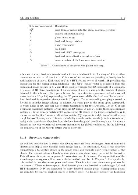
7.1. Map building 115 Sub-map component T W L K I L C Π D A P L Description rigid transformation into the global coordinate system camera calibration matrix plane index image landmark image patches plane covariances 3D planes landmark SIFT descriptors landmark normalization transformations camera matrix of the local coordinate system Table 7.1: Components of the piece-wise planar sub-map. A is a set of size n holding a transformation for each landmark in L. An entry of A is an affine transformation matrix of size 3 × 3. D is a set of feature vectors providing a description for each landmark of size n. Each entry of D is a SIFT feature vector of length 128 providing the description for the corresponding landmark. The SIFT feature vector is computed from the normalized image patches in L. I and Π are used to represent the 3D coordinate of a landmark. Π is a set of 3D plane descriptions of the sub-map of size p, where p is the number of planes detected in the sub-map. Each plane is described by a 6-vector (parameterized with normal vector and one 3D point) representing the 3D parameters within the local coordinate system. Each landmark is located on these planes in 3D space. The corresponding mapping is stored in I which is an index image holding the information which pixel in the image space corresponds to which plane in 3D. The map also contains uncertainties for the 3D planes. The set C of size p contains covariance matrices for the different 3D planes. K and P L define the local coordinate system. P L is the camera matrix which connects the 3D planes to the image coordinates. K is the corresponding 3 × 3 camera calibration matrix. TL W represents a rigid transformation into the global coordinate system. It is a 4×4 similarity transformation matrix (rotation, translation, scale) which transforms 3D points from the local into the global coordinate system. A sub-map defined in that way contains all necessary information for global localization. In the following the computation of the various entries will be described. 7.1.3 Structure computation We will now describe how to extract the 3D map structure from two images. From the sub-map identification step a short-baseline stereo image pair I, I ′ is established. Goal of the structure computation is to identify planes in the image scene and compute a 3D reconstruction of the planes. The reconstruction will only contain planes, non-planar image parts will be discarded. This will result in a piece-wise planar 3D reconstruction of the scene. The segmentation of the scene into planar regions will be done with the method described in Chapter 6. Prerequisite for this method is that the camera poses are known. Thus in a first step the camera positions for the images I, I ′ have to be computed. DoG interest points are detected in both images I, I ′ and SIFT descriptors D, D ′ are computed for every detected interest point. Corresponding points are identified by nearest neighbor search in feature space. As distance measure the Euclidean
7.1. Map building 116 distance is used. Two features correspond if d 01 d 02 < t (7.6) where d 01 is the Euclidean distance between the query feature and the nearest feature point from D ′ and d 02 is the Euclidean distance to the second closest feature. t is a distance threshold. Good results can be achieved with t=0.8. The distance measure has been suggested by Lowe [67] for SIFT feature matching. The such established feature correspondences can now be used for estimating the camera poses. As already mentioned we assume calibrated cameras, i.e. the calibration matrix K is know. Thus we can estimate the essential matrix which encodes the camera positions of the two viewpoints. Essential matrix estimation is performed using the 5- point algorithm of Nister [83] within a standard RANSAC scheme [28]. The essential matrix E can be decomposed into two camera matrices P, P ′ where P is the canonical camera matrix and P ′ defines the second camera position in the local canonical coordinate frame (see equation 7.7 and 7.8). ⎛ ⎞ 1 0 0 0 P = ⎝ 0 1 0 0 ⎠ (7.7) 0 0 1 0 P ′ = [R|t] (7.8) R is a 3 × 3 rotation matrix and t is a translation 3-vector defining the baseline of the stereo case. P, P ′ are input parameters for the subsequent plane segmentation and reconstruction step. The algorithm requires also initial guesses for small planar regions in the images I, I ′ as input parameters with the according inter-image homographies. For that MSER regions are detected in I and I ′ . Region matching is performed (as described in Section 6.1) which returns point correspondences within each interest region and the according homography transform. This constitutes the initial guesses for the plane segmentation algorithm. Plane segmentation and reconstruction is now performed yielding the following map components: • An index image I. • A set of detected and reconstructed planes Π. Each plane is represented by a 6-vector giving the full 3D parameters in the local coordinate frame. • Covariances for each plane giving an uncertainty measure for the reconstruction accuracy. The structure computation will be completed by a post-processing step. Planes which are extended behind the camera planes are removed. This consistency check deletes incorrect reconstructed image parts resulting in higher robustness. The different steps of structure reconstruction are illustrated in Figure 7.3. 7.1.4 Landmark extraction Up to now the sub-map is still missing essential components, the landmarks. Closing this gap is the goal of the next step. Landmark appearance has to be connected to 3D information and incorporated into the sub-map. In the following we describe an approach using MSER interest regions as landmarks. However, the definition of the sub-map is general enough to allow the use of any other kind of interest regions. In the following the necessary steps are outlined:
Page 1 and 2:
Graz University of Technology Insti
Page 3 and 4:
Abstract Visual map building and lo
Page 5 and 6:
Contents 1 Introduction to mobile r
Page 7 and 8:
CONTENTS vi 7.1.5 Sub-map linking .
Page 9 and 10:
1.1. Localization and map building
Page 11 and 12:
1.3. What has already been achieved
Page 13 and 14:
1.5. How can it get solved? 6 fully
Page 15 and 16:
1.6. Contribution of this thesis 8
Page 17 and 18:
1.7. Structure of the thesis 10 com
Page 19 and 20:
2.2. Localization from point featur
Page 21 and 22:
2.2. Localization from point featur
Page 23 and 24:
2.4. Localization from plane featur
Page 25 and 26:
2.5. Summary 18 or not. Clearly thi
Page 27 and 28:
Chapter 3 Local detectors Research
Page 29 and 30:
3.1. Interest point detectors 22 fu
Page 31 and 32:
3.2. Scale invariant detectors 24 r
Page 33 and 34:
3.2. Scale invariant detectors 26 (
Page 35 and 36:
3.2. Scale invariant detectors 28 3
Page 37 and 38:
3.3. Affine invariant detectors 30
Page 39 and 40:
Page 41 and 42:
Page 43 and 44:
Page 45 and 46:
Page 47 and 48:
3.4. Comparison of the described me
Page 49 and 50:
3.4. Comparison of the described me
Page 51 and 52:
44 But using a plane to plane homog
Page 53 and 54:
4.2. Representation of the detectio
Page 55 and 56:
4.3. Detection correspondence 48 th
Page 57 and 58:
4.4. Point transfer using the trifo
Page 59 and 60:
4.5. Ground truth generation 52 usi
Page 61 and 62:
4.6. Experimental evaluation 54 Fig
Page 63 and 64:
4.6. Experimental evaluation 56 rep
Page 65 and 66:
4.6. Experimental evaluation 58 MSE
Page 67 and 68:
4.6. Experimental evaluation 60 mat
Page 69 and 70:
4.6. Experimental evaluation 62 vie
Page 71 and 72: 4.6. Experimental evaluation 64 vie
Page 73 and 74: 4.6. Experimental evaluation 66 rel
Page 75 and 76: Chapter 5 Maximally Stable Corner C
Page 77 and 78: 5.1. The MSCC detector 70 (a) (b) (
Page 79 and 80: 5.2. Region representation 72 400 (
Page 81 and 82: 5.3. Computational complexity 74 6.
Page 83 and 84: 5.5. Detection examples 76 paramete
Page 85 and 86: 5.5. Detection examples 78 Figure 5
Page 87 and 88: 5.6. Detector evaluation: Repeatabi
Page 89 and 90: 5.7. Combining MSCC with other loca
Page 99 and 100: 6.1. Wide-baseline region matching
Page 101 and 102: 6.1. Wide-baseline region matching
Page 103 and 104: 6.2. Piece-wise planar scene recons
Page 117 and 118: Chapter 7 Living in a piecewise pla
Page 119 and 120: 7.1. Map building 112 s,R,t sub-map
Page 121: 7.1. Map building 114 x = (x 1 ...x
Page 125 and 126: 7.1. Map building 118 normalization
Page 127 and 128: 7.2. Localization 120 where N = |D
Page 129 and 130: 7.2. Localization 122 registration
Page 131 and 132: 7.2. Localization 124 (a) (b) (c) F
Page 133 and 134: 7.2. Localization 126 3D structure
Page 135 and 136: 7.2. Localization 128 other landmar
Page 137 and 138: Chapter 8 Map building and localiza
Page 139 and 140: 8.2. Map building experiments 132 8
Page 141 and 142: 8.2. Map building experiments 134 D
Page 143 and 144: 8.2. Map building experiments 136 (
Page 145 and 146: 8.2. Map building experiments 138 F
Page 147 and 148: 8.2. Map building experiments 140 F
Page 149 and 150: 8.3. Localization experiments 142 8
Page 151 and 152: 8.3. Localization experiments 144 F
Page 153 and 154: 8.3. Localization experiments 146 F
Page 155 and 156: 8.3. Localization experiments 148 8
Page 157 and 158: 8.3. Localization experiments 150 (
Page 159 and 160: Chapter 9 Conclusion More than 25 y
Page 161 and 162: 9.1. Future work 154 Map building a
Page 163 and 164: 9.1. Future work 156 information ca
Page 165 and 166: A.1. Projective ellipse transfer 15
Page 167 and 168: A.1. Projective ellipse transfer 16
Page 169 and 170: A.2. Affine approximation of ellips
Page 171 and 172: Appendix B The trifocal tensor and
Page 173 and 174:
Bibliography [1] S. Atiya and G. Ha
Page 175 and 176:
168 [31] F. Fraundorfer and H. Bisc
Page 177 and 178:
170 [61] U. Köthe. Edge and juncti
Page 179 and 180:
172 [92] F. Schaffalitzky and A. Zi
show all

PHD Thesis - Institute for Computer Graphics and Vision - Graz ...

Create successful ePaper yourself

Delete template?

Save as template?