PHD Thesis - Institute for Computer Graphics and Vision - Graz ...

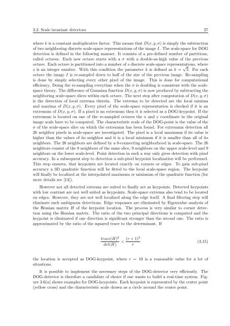
3.2. Scale invariant detectors 27
where k is a constant multiplicative factor. This means that D(x, y, σ) is simply the subtraction
of two neighboring discrete scale-space representations of the image I. The scale-space for DOG
detection is defined in the following manner. It consists of a pre-defined number of partitions,
called octaves. Each new octave starts with a σ with a double-as-high value of the previous
octave. Each octave is partitioned into a number of s discrete scale-space representations, where
s is an integer number. With this condition the parameter k is defined as k = √ 2. For each
octave the image I is re-sampled down to half of the size of the previous image. Re-sampling
is done by simply selecting every other pixel of the image. This is done for computational
efficiency. Doing the re-sampling everytime when the σ is doubling is consistent with the scalespace
theory. The difference of Gaussian function D(x, y, σ) is now produced by subtracting the
neighboring scale-space slices within each octave. The next step after computation of D(x, y, σ)
is the detection of local extrema therein. The extrema to be detected are the local minima
and maxima of D(x, y, σ). Every pixel of the scale-space representation is checked if it is an
extremum of D(x, y, σ). If a pixel is an extremum then it is selected as a DOG-keypoint. If the
extremum is located on one of the re-sampled octaves the x and y coordinate in the original
image scale have to be computed. The characteristic scale of the DOG-point is the value of the
σ of the scale-space slice on which the extremum has been found. For extremum detection all
26 neighbor pixels in scale-space are investigated. The pixel is a local maximum if its value is
higher than the values of its neighbor and it is a local minimum if it is smaller than all of its
neighbors. The 26 neighbors are defined by a 8-connecting neighborhood in scale-space. The 26
neighbors consist of the 8 neighbors of the same slice, 9 neighbors on the upper scale-level and 9
neighbors on the lower scale-level. Point detection in such a way only gives detection with pixel
accuracy. In a subsequent step to detection a sub-pixel keypoint localization will be performed.
This step ensures, that keypoints are located exactly on corners or edges. To gain sub-pixel
accuracy a 3D quadratic function will be fitted to the local scale-space region. The keypoint
will finally be localized at the interpolated maximum or minimum of the quadratic function (for
more details see [13]).
However not all detected extrema are suited to finally act as keypoints. Detected keypoints
with low contrast are not well suited as keypoints. Scale-space extrema also tend to be located
on edges. However, they are not well localized along the edge itself. A final filtering step will
eliminate such ambiguous detections. Edge responses are eliminated by Eigenvalue analysis of
the Hessian matrix H of the keypoint location. The process is very similar to corner detection
using the Hessian matrix. The ratio of the two principal directions is computed and the
keypoint is eliminated if one direction is significant stronger than the second one. The ratio is
approximated by the ratio of the squared trace to the determinant. If
trace(H) 2
det(H)
<
(r + 1)2
r
(3.15)
the location is accepted as DOG-keypoint, where r = 10 is a reasonable value for a lot of
situations.
It is possible to implement the necessary steps of the DOG-detector very efficiently. The
DOG-detector is therefore a candidate of choice if one wants to build a real-time system. Figure
3.6(a) shows examples for DOG-keypoints. Each keypoint is represented by the center point
(yellow cross) and the characteristic scale drawn as a circle around the center point.