PHD Thesis - Institute for Computer Graphics and Vision - Graz ...

7.2. Localization 128
other landmark matches are available to compute the epipolar distance. The other one is using
the lp-score. Both algorithm are very similar up to the scoring function.
Epipolar criteria method
Let us start with landmark extraction and matching. Similar to the sub-map linking step, MSER
regions are extracted from the image of the current view. A LAF is computed for each region
and region normalization is performed. A SIFT-descriptor is computed from the normalized
image patch. Landmark correspondences are detected with the method of section 6.1. The
subsequent pose estimation step requires planar landmarks, thus the planarity has to be checked
for each image region. Non-planar landmarks will be discarded. During map building images are
segmented into piece-wise planar areas. If a landmark is located within the detected planar areas
its planarity is confirmed. The region matching algorithm establishes point correspondences
within the support region of the feature (the area the SIFT-descriptor is computed from). For
each landmark we now compute a set of pose hypotheses Q. For this first 3D − 2D point
correspondences are computed from the 2D − 2D point correspondences by projection onto
the 3D plane. Multiple hypotheses are generated by drawing smaller samples (of size p) from
the whole set of 3D − 2D correspondences. For each of the n random sub-sets S the pose is
computed as follows. First the 5-point algorithm [83] is used to create an initial rotation R
from the 2D − 2D point correspondences. With this initial rotation R the pose is computed
from the 3D − 2D correspondences using the iterative method of Lu and Hager [68]. The pose
hypotheses is added to Q if it represents a valid configuration, i.e. the 3D points are in front of
the camera. This is repeated for all matched landmarks. If all pose hypotheses are created the
epipolar distance is computed for each hypothesis. As resulting pose the one with the smallest
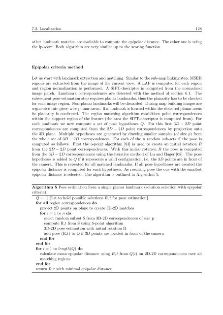
epipolar distance is selected. The algorithm is outlined in Algorithm 5.
Algorithm 5 Pose estimation from a single planar landmark (solution selection with epipolar
criteria)
Q ← [] {list to hold possible solutions R, t for pose estimation}
for all region correspondences do
project 2D points on plane to create 3D-2D matches
for i = 1 to n do
select random subset S from 3D-2D correspondences of size p
compute R,t from S using 5-point algorithm
3D-2D pose estimation with initial rotation R
add pose (R,t) to Q if 3D points are located in front of the camera
end for
end for
for i = 1 to length(Q) do
calculate mean epipolar distance using R, t from Q(i) on 2D-2D correspondences over all
matching regions
end for
return R, t with minimal epipolar distance