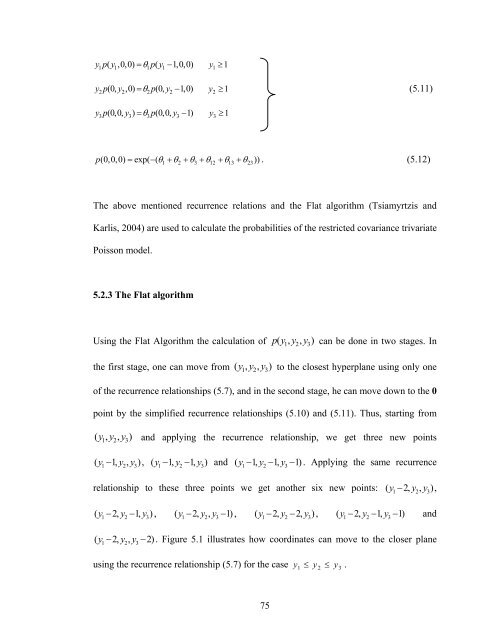
Marginal distributions are Poisson: Y i ~ i ij ik Poisson( θ + θ + θ ) , ⎧i = 1,..., n ⎪ ⎨ jk , = 2,..., n. ⎪ ⎩ jk , ≠ i The joint probability function is given by py ( , y, y; ) = PY [ = yY , = y, Y= y] = (2) ( y − x ) 1 2 θ m (3) m∈ ( y j − xk)! xi! . x A ∏ ∑ ∏ ( j ) j∈R1 k∈R i∈R 2 2 1 2 3 1 1 2 2 3 3 L ∑ ∑ exp( − θ ) ∏ j∈R θ j ∑ j k ( j ) k∈R 2 ∏ i∈R θ xi i The calculation <strong>of</strong> above joint probability function is not easy. Here, we used recurrence relations involving densities to compute the probability function. In 1967, Mahamunulu presented some important notes regarding p variate Poisson distributions. According to him the following recurrence relations are obtained <strong>for</strong> the trivariate two-way covariance model: y p( y , y , y ) = θ p( y − 1, y , y ) + θ p( y −1, y − 1, y ) + θ p( y −1, y , y − 1) (5.7) 1 1 2 3 1 1 2 3 12 1 2 3 13 1 2 3 y p( y , y , y ) = θ p( y , y − 1, y ) + θ p( y −1, y − 1, y ) + θ p( y , y −1, y − 1) (5.8) 2 1 2 3 2 1 2 3 12 1 2 3 23 1 2 3 y p( y , y , y ) = θ p( y , y , y − 1) + θ p( y −1, y , y − 1) + θ p( y , y −1, y − 1) , (5.9) 3 1 2 3 3 1 2 3 13 1 2 3 23 1 2 3 with py ( 1, y2, y 3) = 0 if min{ y1, y2, y 3} < 0. It also gives the following relations: ypy 1 ( 1, y2, 0) = θ1py ( 1− 1, y2, 0) + θ12py ( 1−1, y2− 1, 0) y1, y2 ≥ 1 yp 2 (0, y2, y3) = θ2p(0, y2− 1, y3) + θ23p(0, y2−1, y3− 1) y2, y3 ≥ 1 (5.10) ypy 3 ( 1,0, y3) = θ3py ( 1,0, y3− 1) + θ13py ( 1−1,0, y3− 1) y1, y3 ≥ 1 74
ypy ( ,0,0) = θ py ( − 1,0,0) y1 ≥ 1 1 1 1 1 yp(0, y,0) = θ p(0, y− 1,0) y2 ≥ 1 (5.11) 2 2 2 2 yp(0,0, y) = θ p(0,0, y− 1) y3 ≥ 1 3 3 3 3 p(0,0,0) = exp( − ( θ + θ + θ + θ + θ + θ )) . (5.12) 1 2 3 12 13 23 The above mentioned recurrence relations and the Flat algorithm (Tsiamyrtzis and Karlis, 2004) are used to calculate the probabilities <strong>of</strong> the restricted covariance trivariate Poisson model. 5.2.3 The Flat algorithm Using the Flat Algorithm the calculation <strong>of</strong> py ( 1, y2, y 3) can be done in two stages. In the first stage, one can move from ( y1, y2, y 3) to the closest hyperplane using only one <strong>of</strong> the recurrence relationships (5.7), and in the second stage, he can move down to the 0 point by the simplified recurrence relationships (5.10) and (5.11). Thus, starting from ( y1, y2, y 3) and applying the recurrence relationship, we get three new points ( y1− 1, y2, y3) , ( y1−1, y2− 1, y3) and ( y 1 −1, y 2 −1, y 3 − 1) . Applying the same recurrence relationship to these three points we get another six new points: ( y 1 − 2, y 2 , y 3 ), ( y1−2, y2− 1, y3) , ( y1−2, y2, y3− 1) , ( y1− 2, y2− 2, y3) , ( y1−2, y2−1, y3− 1) and ( y −2, y , y − 2) . Figure 5.1 illustrates how coordinates can move to the closer plane 1 2 3 using the recurrence relationship (5.7) <strong>for</strong> the case y1 ≤ y2 ≤ y3 . 75
- Page 1 and 2:
MULTIVARIATE POISSON HIDDEN MARKOV
- Page 3 and 4:
ABSTRACT Multivariate count data ar
- Page 5 and 6:
ACKNOWLEDGEMENT First I would like
- Page 7 and 8:
TABLE OF CONTENTS PERMISSION TO USE
- Page 9 and 10:
6.4 Data analysis..................
- Page 11 and 12:
Table 7.7: Loglikelihood and AIC to
- Page 13 and 14:
Figure 6.10: Loglikelihood, AIC and
- Page 15 and 16:
CHAPTER 1 GENERAL INTRODUCTION 1.1
- Page 17 and 18:
North Carolina, is modelled by Symo
- Page 19 and 20:
concept of Markov models to include
- Page 21 and 22:
egularity constraints on the underl
- Page 23 and 24:
CHAPTER 2 HIDDEN MARKOV MODELS ( HM
- Page 25 and 26:
Given the coin tossing experiment,
- Page 27 and 28:
P 11 P 22 P 12 1 2 P 21 P 32 P 13 P
- Page 29 and 30:
0.8 0.6 0.2 1 0.4 2 (1) P [H]=2/3 (
- Page 31 and 32:
… Urn 1 Urn 2 Urn N P[Red]= b 1 (
- Page 33 and 34:
5. The probability distribution of
- Page 35 and 36:
focus of this section. Random field
- Page 37 and 38: Now consider a random field { X ( s
- Page 39 and 40: for some real β . Again, the denom
- Page 41 and 42: Since original HMMs were designed a
- Page 43 and 44: CHAPTER 3 INFERENCE IN HIDDEN MARKO
- Page 45 and 46: sequence. If we have several compet
- Page 47 and 48: Using this equation we can calculat
- Page 49 and 50: 3.2.2 Problem 2 and its solution Gi
- Page 51 and 52: Letting Ut( S1 = i1, S2 = i2,..., S
- Page 53 and 54: ξ α () iPβ ( jb ) ( y ) t ij t+
- Page 55 and 56: ˆ ( n) = b j Expected Number of ti
- Page 57 and 58: CHAPTER 4 HIDDEN MARKOV MODEL AND T
- Page 59 and 60: 4.2.1 Wild Oats Figure 4.1: Wild Oa
- Page 61 and 62: 4.2.2.1 Effects on crop quality Wil
- Page 63 and 64: at each of the 150 grid locations (
- Page 65 and 66: In the literature review (section 1
- Page 67 and 68: estimated through the observations
- Page 69 and 70: CHAPTER 5 MULTIVARIATE POISSON DIST
- Page 71 and 72: Y Y Y 1 2 3 = X = X 1 = X 2 3 + X +
- Page 73 and 74: educe the computational burden; how
- Page 75 and 76: and y 3 as illustrated above. Again
- Page 77 and 78: q In general, the number of paramet
- Page 79 and 80: Similar to the fully structured mod
- Page 81 and 82: ecause the former captures more of
- Page 83 and 84: (Tsiamyrtzis and Karlis, 2004). The
- Page 85 and 86: notation, the following recursive s
- Page 87: 5.2.2 The multivariate Poisson dist
- Page 91 and 92: ecurrence relationship ypy 1 ( 1 ,
- Page 93 and 94: Raftery, 1998); identification of t
- Page 95 and 96: maximization (EM) algorithm is appl
- Page 97 and 98: the EM algorithms for use on very l
- Page 99 and 100: Another alternative is to use the p
- Page 101 and 102: 5.3.5 Estimation for the multivaria
- Page 103 and 104: j j E[ X 12 i | Yi , Z ij = 1, Φ ]
- Page 105 and 106: 5.4 Multivariate Poisson hidden Mar
- Page 107 and 108: where P = Pr( S = k | S − 1 j), 1
- Page 109 and 110: P jk n ∑ vˆ jk i= 2 = n m ∑∑
- Page 111 and 112: E[ X | Y, u ( i) = 1, Φ ] = d = y
- Page 113 and 114: The bootstrap method is a powerful
- Page 115 and 116: eplications are generally sufficien
- Page 117 and 118: Y and assumes a probability distrib
- Page 119 and 120: For the case of two categorical var
- Page 121 and 122: ejected. In this situation, the (sm
- Page 123 and 124: the Poisson distribution is well su
- Page 125 and 126: 0 1 2 3 4 Wild Buckwheat species109
- Page 127 and 128: Table 6.4: The frequency of occurre
- Page 129 and 130: 6.4.1 Results for the different mul
- Page 131 and 132: Proportion 1.0 0.9 0.8 0.7 0.6 0.5
- Page 133 and 134: -600 -650 -700 Loglikelihood -750 -
- Page 135 and 136: Figure 6.7 illustrates the evolutio
- Page 137 and 138: Table 6.8: Parameter estimates (boo
- Page 139 and 140:
common covariance and the four stat
- Page 141 and 142:
-600 -700 -800 Loglikelihood -900 -
- Page 143 and 144:
Table 6.11: Parameter estimates (bo
- Page 145 and 146:
6.5 Comparison of the different mod
- Page 147 and 148:
loglikelihood providing at least a
- Page 149 and 150:
illustrates the contour plot of the
- Page 151 and 152:
(a) Independent Contour 1 Contour 2
- Page 153 and 154:
Karlis and Meligkotsidou (2006) dis
- Page 155 and 156:
The mean vector and the covariance
- Page 157 and 158:
The simple moments of B are polynom
- Page 159 and 160:
and E ( Y ) = AM where ⎡λ1 ⎤
- Page 161 and 162:
7.5 Applications In addition to wee
- Page 163 and 164:
The estimated covariance matrix and
- Page 165 and 166:
The estimated covariance matrix (AI
- Page 167 and 168:
Table 7.6 Bacterial counts by 3 sam
- Page 169 and 170:
Table 7.8: Loglikelihood and AIC to
- Page 171 and 172:
(c) Finite mixture with the five co
- Page 173 and 174:
(i) Hidden Markov model with the fi
- Page 175 and 176:
CHAPTER 8 COMPUTATIONAL EFFICIENCY
- Page 177 and 178:
less time compared to the multivari
- Page 179 and 180:
1400 1200 CPU time (1/100 second) 1
- Page 181 and 182:
1400 1200 CPU time (1/100 second) 1
- Page 183 and 184:
In this thesis, three species count
- Page 185 and 186:
In the applications of the HMMs, li
- Page 187 and 188:
indication of the relative goodness
- Page 189 and 190:
underlying data. The advantage of t
- Page 191 and 192:
9.6 Further research We can present
- Page 193 and 194:
REFERENCES 1. Aas, K., Eikvil, L. a
- Page 195 and 196:
17. Bicego, M., Murino, V. & Figuei
- Page 197 and 198:
33. Descombes, X., Morris, R.D., Ze
- Page 199 and 200:
Department of Statistics, Universit
- Page 201 and 202:
66. Li C.S., Lu J.C., Park J., Kim
- Page 203 and 204:
85. Petrie T. (1969). Probabilistic
- Page 205 and 206:
104. University of Manitoba, Depart
- Page 207 and 208:
z0
- Page 209 and 210:
threep2[i]
- Page 211 and 212:
loglike[nit]
- Page 213 and 214:
theta33
- Page 215 and 216:
} prob[g1+1, g2 + 1]
- Page 217 and 218:
theta131
- Page 219 and 220:
threep22[i]
- Page 221 and 222:
dens=matrix(0,nrow=T,ncol=N) alpha=
- Page 223 and 224:
# vˆ jk ( i) = P jk f ( y ; λ i