Weeki Wachee River System Recommended Minimum Flows and ...

More documents

Recommendations

Info

explains, the energy plot shows the relative portion of the data explained by the individual wavelets (energy being the sum of the squares of the wavelet coefficients). In Figure 4 there appear to be two clusters within each of the energy plots. One cluster represents higher frequency components of the data and the other cluster represents the lower frequency components. Since we are concerned primarily with the long term behavior the lower frequency components of were extracted from both the flow and rainfall data. bville.vec -10 0 10 20 Brooksville Centered Rainfall 1941 1946 1951 1956 1961 1966 1971 1976 1981 1986 1991 1996 2001 Discrete Wavelet Transform of Rainfall bville.vec d1 d2 d3 d4 d5 s5 1941 1946 1951 1956 1961 1966 1971 1976 1981 1986 1991 1996 2001 Figure 3 Brooksville Rainfall and Transformed Rainfall Figure 5 shows the original flow data and the results of filtering using the untransformed set of "d4" through "s5" wavelets. From the graph it is obvious that what has been accomplished is that the data has been smoothed. Similar results could have been obtained using loess, W eeki W achee Flow B ro o ks v ille R a in fa ll Data Data d1 d1 d2 d2 d3 d3 d4 d4 d5 d5 s5 s5 0.0 0.2 0.4 0.6 0.8 1.0 0.0 0.2 0.4 0.6 0.8 1.0 Energy (100% ) Energy (100%) Figure 4 Wavelet Energy Diagrams ____________________________________________________________________________________________ Proposed Minimum Flows and Levels for Weeki Wachee River Page 127 of 164 Appendices
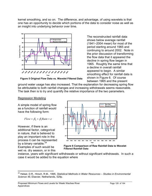
kernel smoothing, and so on. The difference, and advantage, of using wavelets is that one has an opportunity to decide which portions of the data to consider noise as well as an insight into underlying behavior over time. Centered Flow (cfs) 100 80 60 40 20 0 -20 -40 -60 1941 1945 1949 1953 1957 1961 1965 1969 1973 The reconstructed rainfall data shows below average rainfall (1941–2004 mean) for most of the period starting around 1965 and continuing to around 2002. Note in the prior discussion of transforming the flow data that it appeared the decline in spring flow began in 1965. Roughly the same time that a decline in overall rainfall appeared to begin. A similar smoothing effect for rainfall data is shown in Figure 6. Of course between 1965 and the present ground water usage has also increased. That the explanation for decreasing spring flow be attributable to both rainfall changes and increasing withdrawals seems reasonable. The task then is to try and quantify the relative importance of the two parameters. Regression Modeling Year A simple model of spring flow as a function of rainfall would have the following form: Flow = β 0 + β1Rain + ε However, if there is an additional factor, categorical in nature, that is believed to play an important role in the process it can be represented by a binary variable. 29 Examples of such would be wet vs. dry season, or in this Original Data Wavelet Filtered Data 1977 1981 1985 1989 1993 1997 2001 Figure 5 Original Flow Data vs. Wavelet Filtered Data Centered Rainfall 20 10 0 -10 -20 1941 1946 1951 1956 1961 1966 1971 1976 1981 1986 1991 1996 2001 instance, years with significant withdrawals or without significant withdrawals. In such a case it would be added to the equation where Year Raw Data Wavelet Filtered Figure 6 Comparison of Raw Rainfall Data to Wavelet Filtered Rainfall Data 29 Helsel, D.R., Hirsch, R.M., 1995, Statistical Methods in Water Resources – Studies in Environmental Science 49, Elsevier, Netherlands, 529p. ____________________________________________________________________________________________ Proposed Minimum Flows and Levels for Weeki Wachee River Page 128 of 164 Appendices
Page 1:
Weeki Wachee River System Recommend
Page 4 and 5:
Conversion Table Metric to U.S. Cus
Page 6 and 7:
5.2 FISH ..........................
Page 8 and 9:
Figure 3-2 Location of Bathymetric
Page 10 and 11:
LIST OF TABLES Table 1-1 Rule-of-Th
Page 12 and 13:
Table 8-1 Summary of Weeki Wachee M
Page 14 and 15:
Executive Summary Minimum Flows and
Page 16 and 17:
CHAPTER 1 - PURPOSE & BACKGROUND OF
Page 18 and 19:
1) flood flows that determine the b
Page 20 and 21:
the area." What constitutes "signif
Page 22 and 23:
Table 1-1 Rule-of-Thumb Estimates f
Page 24 and 25:
this report identifies specific res
Page 26 and 27:
1.6 Content of Remaining Chapters I
Page 28 and 29:
CHAPTER 2 - WATERSHED CHARACTERISTI
Page 30 and 31:
# # # circular vent 1.8 meters in d
Page 32 and 33:
Figure 2-5 1970s Aerial with 1999 U
Page 34 and 35:
is a variation of the Seminole word
Page 36 and 37:
Figure 2-6 Hurricane Tracks near Ba
Page 38 and 39:
varied by period. The variation was
Page 40 and 41:
2.3.2 Baseline Period Figure 2-10 i
Page 42 and 43:
found (ktau p=0.06) between total g
Page 44 and 45:
similarly across the springsheds ex
Page 46 and 47:
Figure 2-15 Wavelet Filtered Discha
Page 48 and 49:
Figure 2-16 INTB Groundwater Model
Page 50 and 51:
2.6 Seasonal Blocks As described in
Page 52 and 53:
Table 2-6 Median (cfs) Flow by Bloc
Page 54 and 55:
# # # Surface waters in this stretc
Page 56 and 57:
3.1.3 Segmentation Segmentation was
Page 58 and 59:
Figure 3-5 Dominant SAV and Median
Page 60 and 61:
Figure 3-6 Sediment Characteristics
Page 62 and 63:
Figure 3-7 Shoreline / Buffer Veget
Page 64 and 65:
CHAPTER 4 - TIDE, SALINITY & WATER
Page 66 and 67:
Two additional harmonic pairs were
Page 68 and 69:
Figure 4-5. Median Bottom Salinity
Page 70 and 71:
Figure 4-7 Salinity Range (1984-200
Page 72 and 73:
uncovering in response to strong wi
Page 74 and 75:
E) Salinity = β o + β 1 *Flow 2 +
Page 76 and 77:
Additional exploratory attempts usi
Page 78 and 79:
86 = 186 cfs, SWFWMD 1994-96 = 167
Page 80 and 81:
A regression of the form below was
Page 82 and 83:
Table 4-8 Median Water Quality of W
Page 84 and 85:
Figure 4-10 Nitrate Concentration a
Page 86 and 87:
CHAPTER 5 - BIOLOGICAL CHARACTERIST
Page 88 and 89:
Figure 5-1 Principal Component Anal
Page 90 and 91:
measured volume sampled which was t
Page 92 and 93: 5.2.2 Relation to inflow Response t
Page 94 and 95: Table 5-7 Location Response (km u )
Page 96 and 97: Table 5-9 Abundance Response to Inf
Page 98 and 99: animals can survive chronic exposur
Page 100 and 101: Figure 5-3 Number of Aerial Manatee
Page 102 and 103: Figure 5-5(a) Molluscan Presence /
Page 104 and 105: Table 5-11 Rank Order of Mollusc Ab
Page 106 and 107: Figure 5-5 Polymesoda caroliniana A
Page 108 and 109: Figure 6-1 Plankton Tow Flows Compa
Page 110 and 111: In application, a baseline area and
Page 112 and 113: 6.1.4 Benthos Protection for benthi
Page 114 and 115: Figure 6-3. Location of the Three P
Page 116 and 117: 7.2 Manatee Approach Establishing a
Page 118 and 119: Figure 7-2 Joint Probability of Occ
Page 120 and 121: Figure 7-3 Maximum Day Manatee Usag
Page 122 and 123: Figure 7- 6 Example Calculations fo
Page 124 and 125: Figure 7- 7 Estimation of Flow Redu
Page 126 and 127: Figure 7-8. Summary Results for the
Page 128 and 129: The reductions in flow that meet th
Page 130 and 131: probably accounts in part for the d
Page 132 and 133: Postel, S. and B.Richter. 2003. Riv
Page 134 and 135: Stanford, J.A., J.V.Ward, W.J. Liss
Page 136 and 137: Culter, J.K. 1986. Water Chemistry.
Page 138 and 139: CHAPTER 10 - APPENDICES 10.1 Append
Page 140 and 141: The wavelet used is the symmlets wa
Page 144 and 145: 0 if no significant withdrawal Z =
Page 146 and 147: One advantage of using this regress
Page 148 and 149: Technical Memorandum January 22, 20
Page 150 and 151: Lecanto 1 & 2 #S Well Site Descript
Page 152 and 153: Figure 4. HSPF subbasins in the INT
Page 154 and 155: Most of the limestone mines located
Page 156 and 157: 3.1.3 Septic Tank Recharge in the S
Page 158 and 159: Figure 10. Groundwater grid in the
Page 160 and 161: Basso, R.J., 2004, Hydrogeologic Se
Page 162 and 163: 10.2 Appendices - Chapter 3 Appendi
Page 164 and 165: 10.3 Appendices - Chapter 4 Appendi
Page 166 and 167: Appendix 4-2 Data Sources Water qua
Page 168 and 169: Appendix 4-3 Water Quality Trend Gr
Page 170 and 171: Water Quality Trend Graphics, conti
Page 180 and 181: United States Department of the Int
Page 182 and 183: October 8,2008 Florida Fish and Wil
Page 184 and 185: Martin Kelly, Ph.D. Page 3 October
Page 186 and 187: Scientific Peer Review of the Propo
Page 188 and 189: Determining a low flow need during
Page 190 and 191: Current state water policy, as expr
Page 192 and 193:
Spring, Twin Dees Spring and possib
Page 194 and 195:
under varying flow regimes. The fir
Page 196 and 197:
Weeki Wachee Rainfall, Springflow a
Page 198 and 199:
6.0 Discharge:Precipitation (cfs/in
Page 200 and 201:
Nevertheless, a major concern with
Page 202 and 203:
system grid is not totally orthogon
Page 204 and 205:
In a hydrodynamic model study, one
Page 206 and 207:
analysis was rather cursory. The Di
Page 208 and 209:
(taxa) richness in the WWRS. If the
Page 210 and 211:
Freshwater Habitats Approximately 1
Page 212 and 213:
ERRATA and EDITORIAL COMMENTS Page
Page 214 and 215:
Page Paragraph Line Comment 14 Some
Page 216 and 217:
Page Paragraph Line Comment 21 The
Page 218 and 219:
Page Paragraph Line Comment 26 The
Page 220 and 221:
REFERENCES Alber, M. 2002. A Concep
Page 222 and 223:
Richter, B. D., J. V. Baumgartner,
Page 224 and 225:
the regression equation used to pre
Page 226 and 227:
and the three independent approache
Page 228 and 229:
The Southwest Florida Water Managem
Page 230 and 231:
the model in terms of tides, salini
Page 232 and 233:
Attachment 1 - Comparison of salini
Page 234 and 235:
Figure 1. Predicted drawdown (feet)
show all

Weeki Wachee River System Recommended Minimum Flows and ...

Create successful ePaper yourself

Delete template?

Save as template?