Weeki Wachee River System Recommended Minimum Flows and ...

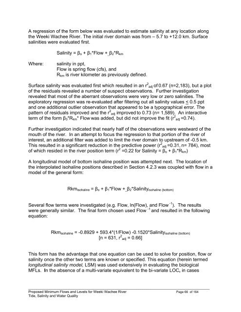
A regression of the form below was evaluated to estimate salinity at any location along
the Weeki Wachee River. The initial river domain was from – 5.7 to +12.0 km. Surface
salinities were evaluated first.
Salinity = β o + β 1 *Flow + _ β 2 *R km
Where:
salinity in ppt,
Flow is spring flow (cfs), and
R km is river kilometer as previously defined.
Surface salinity was evaluated first which resulted in an r 2 adj of 0.67 (n=2,183), but a plot
of the residuals revealed a number of suspect observations. Further investigation
revealed that most of the aberrant observations were very low or zero salinities. The
exploratory regression was re-evaluated after filtering out all salinity values < 0.5 ppt
and one additional outlier observation that appeared to be a typographical error. The
pattern of residuals improved and the r 2 adj improved to 0.73 (n= 1,589). An interactive
term of the form β 3 *R km * Flow was added, but did not improve the fit (r 2 adj =0.74).
Further investigation indicated that nearly half of the observations were westward of the
mouth of the river. In an attempt to focus the regression to that portion of the river of
interest, an additional filter was added to limit the river domain to upstream of -0.5 km.
This resulted in a significant reduction in the predictive power (r 2 adj =0.31, n= 784), most
of which resided in the river position term (r 2 =0.22 for Salinity = β o + β 1 *R km )
A longitudinal model of bottom isohaline position was attempted next. The location of
the interpolated isohaline positions described in Section 4.2.3 was coupled with flow in a
model of the general form:
Rkm isohaline = β o + β 1 *Flow + _ β 2 *Salinity isohaline (bottom)
Several flow terms were investigated (e.g. Flow, ln(Flow), and Flow -1 ). The results
were generally similar. The final form chosen used Flow -1 and resulted in the following
equation:
Rkm isohaline = -0.8929 + 593.4*(1/Flow) -0.1520*Salinity isohaline (bottom)
[n = 631, r 2 adj = 0.66]
This form has the advantage that one equation can be used to solve for position, flow or
salinity once the other two terms are known or specified. This equation (herein termed
longitudinal salinity model, LSM) was used extensively in evaluating the biological
MFLs. In the absence of a multi-variate equivalent to the bi-variate LOC, in cases
____________________________________________________________________________________________
Proposed Minimum Flows and Levels for Weeki Wachee River Page 66 of 164
Tide, Salinity and Water Quality