a review - Acta Technica Corviniensis

1.
István BÍRÓ
SIMPLE NUMERICAL METHOD FOR 2-DOF PLANAR KINETICAL
PROBLEMS
1.
TECHNICAL INSTITUTE, FACULTY OF ENGINEERING, UNIVERSITY OF SZEGED, H-6724 SZEGED, MARS SQ. 7, HUNGARY
ABSTRACT: The motion analysis is an important field in the education of mechanical
engineers. Kinematical and kinetical analysis of rigid bodies linked to each other by
different constraints (mechanical systems) leads to integration of second order
differential equations. In this way the kinematical functions of parts of mechanical
systems can be determined. The degrees of freedom of the mechanical system increase
as a result of the application of elastic parts in it. Numerical methods can be applied
to solve such problems. A simple numerical method will be demonstrated by author by
the aid of several examples. Some parts of results obtained by using the numerical
method were checked by analytical way. The published method can be used in the
technical higher education.
KEYWORDS: rigid bodies, motion analysis, kinematical functions
INTRODUCTION
The knowledge of motion analysis plays an important
role in the education of mechanical engineers.
Dynamical analysis of mechanical systems is a
fundamental chapter in motion analysis. Mechanical
systems having one or two degrees of freedom can be
described by second order differential equations or
differential equation systems. Analytical solution of
them in most cases is quite difficult or impossible.
In such cases the application of numerical methods is
advantage. The results obtained in this way can be
demonstrated in different kinematical diagrams. It
helps engineer students better learning of schoolwork
and connections among different physical
quantities. In this paper the results of kinetical
analysis of two mechanical systems will be
demonstrated.
THE SIMPLE NUMERICAL METHOD
Let us suppose that the mechanical system can be
described by q = q( r,
ϕ)
generalized coordinates.
Physical quantities r & , r ,ϕ&
, ϕ
o o o o
describe the initial
state of the system. Time step: ti+1 − ti
. Applied
algorithms can be seen in table below.
Table 1. Applied algorithms
t & r ( r&
, r,
ϕ& , ϕ)
r& r
t r&
r&
, r , ϕ& , ϕ ) r&
o
1
&
o( o o o o
o
&
1( r&
1,
r1
, ϕ&
1,
ϕ r (
1 1
= r&
o
+ & r
o
t 1
−t
o
&
2( r&
2,
r2
, ϕ&
2,
ϕ2
r2 = r&
1
+ & r
1( t2
−t1
t r ) & ) r = r + r&
t −t
)
2
r
o
1 o o
( 1 o
r2 = r1
+ r&
1( t2
−t1
t r ) & )
)
t …. …. ….
3
t
4
…. …. ….
Table 2. Applied algorithms
t &
ϕ ( r &,
r,
& ϕ,
ϕ)
ϕ& ϕ
t & ϕ r&
, r , & ϕ , ϕ )
o
1
&
o( o o o o
ϕ&
o
&
ϕ (&
1 1,
r1
, & ϕ1,
ϕ1
ϕ 1
= & ϕ o
+ && ϕ o
( t 1
−t
o
&
ϕ (&
2 2,
r2
, & ϕ2,
ϕ2
ϕ
2
= & ϕ1
+ && ϕ1
( t2
−t1
ϕ
o
t r ) & ) ϕ = ϕ + & ϕ t −t
)
2
1 o o
( 1 o
2
= ϕ1
+ ϕ1
( t2
−t1
t r ) & ) ϕ & )
t …. …. ….
3
t
4
…. …. ….
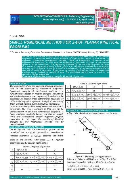
EXAMPLE 1: SPRING PENDULUM (DOF: 2)
In Fig. 1 the sketch of spring pendulum can be seen.
Figure 1. Sketch of spring pendulum
Data: M = -1 Nm, s = 800 N/m, m = 2 kg, R = 0,2 m
(length of unloaded rod), g = 10 m/s 2 , r& o
= 0m/
s,
r = 0, 28m , ϕ&
o
= 0rad/
s, ϕ
o
= 1rad
(time step: 0.0001 s, time interval: 0 ≤ t ≤ 1 s)
© copyright FACULTY of ENGINEERING ‐ HUNEDOARA, ROMANIA 109