a review - Acta Technica Corviniensis

ACTA TECHNICA CORVINIENSIS – Bulletin of Engineering
(Nwachukwu, 2005). Depending upon the type of data
available, the water availability can be computed
from one of the following method, namely; direct
observation method and rain-fall run-off series
method.
STREAM FLOW DATA ANALYSIS
The main objective of stream flow record analysis in
SHP development is to prepare a flow duration curve
and then determine design flow, installed capacity,
plant capacity factor and average discharge.
In order to ascertain how often flow of a given
magnitude occurred during the period of record, a
flow duration curve is prepared. From available data,
the discharge is plotted as ordinate against the
percent of time that discharge is exceeded on the
abscissa and this can be of daily, mean monthly or
mean annual flows.
Flow duration curves from long-term monthly stream
flow records offer a convenient tool in plant capacity
design (Nwachukwu, 2005).
The procedure used to prepare a flow-duration curve
is as follows, demonstrated with a case study of Osun
River.
Table 1: Mean monthly stream flow (m 3 /s) of Osun River
YEAR JAN FEB MAR APR MAY JUNE
1979 84 89 74 97 158 127
1980 74 59 49 69 159 262
1981 42 58 76 111 228 176
1982 65 69 93 82 150 266
1983 73 132 62 116 154 144
1984 33 64 42 97 140 129
1985 105 97 42 67 114 132
YEAR JULY AUG SEP OCT NOV DEC
1979 89 56 48 47 72 136
1980 108 69 47 110 114 81
1981 118 66 47 46 65 65
1982 187 82 55 42 96 76
1983 129 68 42 84 145 155
1984 104 62 43 56 55 51
1985 144 75 50 35 23 24
The discharge in the range 0 to 300m 3 /s has been
divided into 15 classes of 20m 3 /s each as shown in
column1 in table 2. The data are scanned through and
each item is noted in the class group in which it
belongs. The total in each class is shown in column 2.
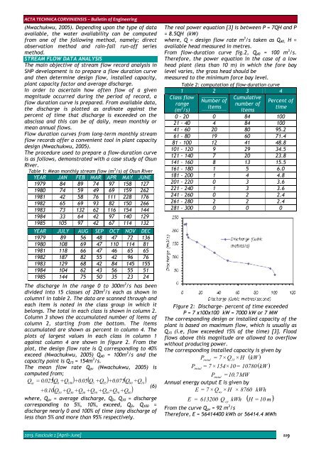
Column 3 shows the accumulated number of items of
column 2, starting from the bottom. The items
accumulated are shown as percent in column 4. The
plots of largest values in each class in column 1
against column 4 are shown in figure 2. From the
plot, the design flow rate is Q corresponding to 40%
exceed (Nwachukwu, 2005) Q 40 = 100m 3 /s and the
capacity point is Q 15 = 154m 3 /s.
The mean flow rate Q av (Nwachukwu, 2005) is
computed from;
Q ( ) ( ) ( )
ay
= 0.025Q0
+ Q100
+ 0.05 Q5
+ Q95
+ 0.075 Q90
+ Q10
(6)
+ 0.10Q ( )
20
+ Q30
+ Q40
+ Q50
+ Q60+
Q70
+ Q80
where, Q av = average discharge, Q 5 , Q 10 = discharge
corresponding to 5%, 10%, exceed, Q 0 , Q 100 =
discharge nearly 0 and 100% of time (any discharge of
less than 5% and more than 95% respectively.
The real power equation [3] is between P = 7QH and P
= 8.5QH (kW)
where, Q = design flow rate m 3 /s taken as Q 40, H =
available head measured in metres.
From flow-duration curve fig.2, Q 40 = 100 m 3 /s.
Therefore, the power equation in the case of a low
head plant (less than 10 m) in which the fore bay
level varies, the gross head should be
measured to the minimum force bay level.
Table 2: computation of flow-duration curve
1 2 3 4
Class flow
range
(m 3 /s)
Number of
items
Cumulative
number of
items
Percent of
time
0 – 20 0 84 100
21 – 40 4 84 100
41 – 60 20 80 95.2
61 – 80 19 60 71.4
81 – 100 12 41 48.8
101 – 120 9 29 34.5
121 – 140 7 20 23.8
141 – 160 8 13 15.5
161 – 180 1 5 6.0
181 – 200 1 4 4.8
201 – 220 0 3 3.6
221 – 240 1 3 3.6
241 – 260 0 2 2.4
261 – 280 2 2 2.4
281 – 300 0 0 0
Figure 2: Discharge– percent of time exceeded
P = 7 x100x100 kW = 7000 kW or 7 MW
The corresponding design or installed capacity of the
plant is based on maximum flow, which is usually as
Q 15 (i.e, flow exceeded 15% of the time) [3]. Flood
flows above this magnitude are allowed to overflow
without producing power.
The corresponding installed capacity is given by
Pinstal = 7 × Q15
× H
P instal
= 7 × 154×
10 =
P instal
= 10.7MW
Annual energy output E is given by
E = 7 × Qay × H × 8760
( kW )
10780 ( kW )
kWh
( )
E = 613200 Q
ay
kWh H = 10 m
From the curve Q av = 92 m 3 /s
Therefore, E = 56414400 kWh or 56414.4 MWh
2013. Fascicule 2 [April–June] 119