Interim Report - TEEB

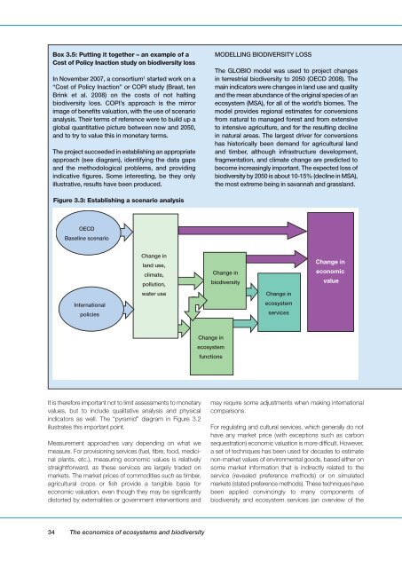
Box 3.5: Putting it together – an example of a
Cost of Policy Inaction study on biodiversity loss
In November 2007, a consortium 1 started work on a
“Cost of Policy Inaction” or COPI study (Braat, ten
Brink et al. 2008) on the costs of not halting
biodiversity loss. COPI’s approach is the mirror
image of benefits valuation, with the use of scenario
analysis. Their terms of reference were to build up a
global quantitative picture between now and 2050,
and to try to value this in monetary terms.
The project succeeded in establishing an appropriate
approach (see diagram), identifying the data gaps
and the methodological problems, and providing
indicative figures. Some interesting, be they only
illustrative, results have been produced.
MODELLING BIODIVERSITY LOSS
The GLOBIO model was used to project changes
in terrestrial biodiversity to 2050 (OECD 2008). The
main indicators were changes in land use and quality
and the mean abundance of the original species of an
ecosystem (MSA), for all of the world’s biomes. The
model provides regional estimates for conversions
from natural to managed forest and from extensive
to intensive agriculture, and for the resulting decline
in natural areas. The largest driver for conversions
has historically been demand for agricultural land
and timber, although infrastructure development,
fragmentation, and climate change are predicted to
become increasingly important. The expected loss of
biodiversity by 2050 is about 10-15% (decline in MSA),
the most extreme being in savannah and grassland.
Figure 3.3: Establishing a scenario analysis
OECD
Baseline scenario
International
policies
Change in
land use,
climate,
pollution,
water use
Change in
biodiversity
Change in
ecosystem
services
Change in
economic
value
Change in
ecosystem
functions
It is therefore important not to limit assessments to monetary
values, but to include qualitative analysis and physical
indicators as well. The “pyramid” diagram in Figure 3.2
illustrates this important point.
Measurement approaches vary depending on what we
measure. For provisioning services (fuel, fibre, food, medicinal
plants, etc.), measuring economic values is relatively
straightforward, as these services are largely traded on
markets. The market prices of commodities such as timber,
agricultural crops or fish provide a tangible basis for
economic valuation, even though they may be significantly
distorted by externalities or government interventions and
may require some adjustments when making international
comparisons.
For regulating and cultural services, which generally do not
have any market price (with exceptions such as carbon
sequestration) economic valuation is more difficult. However,
a set of techniques has been used for decades to estimate
non-market values of environmental goods, based either on
some market information that is indirectly related to the
service (revealed preference methods) or on simulated
markets (stated preference methods). These techniques have
been applied convincingly to many components of
biodiversity and ecosystem services (an overview of the
34 The economics of ecosystems and biodiversity