
Create successful ePaper yourself
Turn your PDF publications into a flip-book with our unique Google optimized e-Paper software.
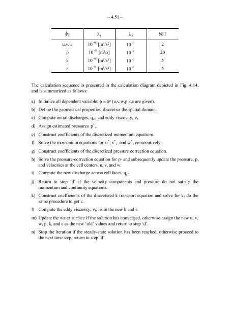
– 4.51 –<br />
��<br />
�� �� �� NIT<br />
u,v,w 10 �6 [m 4 /s 2 ] 10 �3 2<br />
p 10 �5 [m 3 /s] 10 �2 20<br />
k� 10 �6 [m 5 /s 3 ] 10 �3 5<br />
� 10 �6 [m 5 /s 4 ] 10 �3 5<br />
The calculation sequence is presented in the calculation diagram depicted in Fig. 4.14,<br />
and is summarized as follows:<br />
a) Initialize all dependent variable: ����� o �(u,v,w,p,k,� are given).<br />
b) Define the geometrical properties, discretise the spatial domain.<br />
c) Compute initial discharges, qcf, and eddy viscosity, �t.<br />
d) Assign estimated pressures p � ,.<br />
e) Construct coefficients of the discretized momentum equations.<br />
f) Solve the momentum equations for u � , v � , and w � , consecutively.<br />
g) Construct coefficients of the discretized pressure correction equation.<br />
h) Solve the pressure-correction equation for p c and subsequently update the pressure, p,<br />
and velocities at the cell centers, u, v, and w.<br />
i) Compute the new discharge across cell faces, q cf .<br />
j) Return to step ‗d‘ if the velocity components and pressure do not satisfy the<br />
momentum and continuity equations.<br />
k) Construct coefficients of the discretized k transport equation and solve for k; do the<br />
same procedure to get �.<br />
l) Compute the eddy viscosity, �t, from the new k and �<br />
m) Update the water surface if the solution has converged, otherwise assign the new u, v,<br />
w, p, k, and � as the new ‗old‘ values and return to step ‗d‘.<br />
n) Stop the iteration if the steady-state solution has been reached, otherwise proceed to<br />
the next time step, return to step ‗d‘.