Thesis High-Resolution Photoemission Study of Kondo Insulators ...

More documents

Recommendations

Info

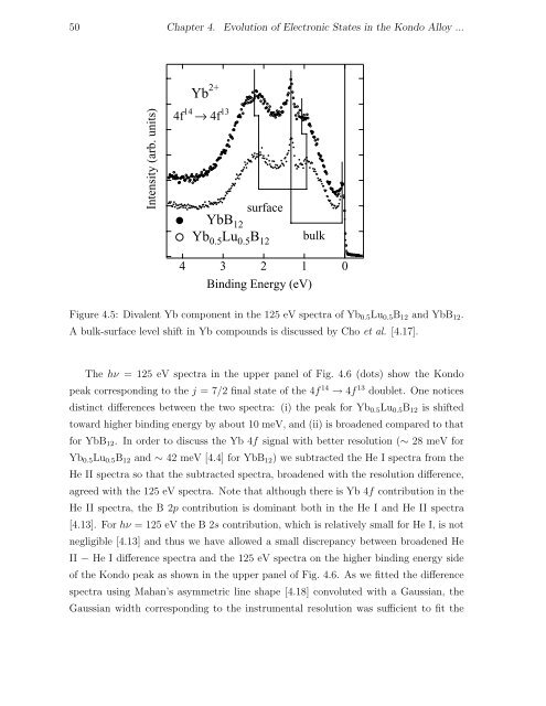
50 Chapter 4. Evolution of Electronic States in the Kondo Alloy ... Intensity (arb. units) Yb 2+ 4f 14 → 4f 13 surface YbB12 Yb0.5Lu0.5B12 4 3 2 1 0 Binding Energy (eV) bulk Figure 4.5: Divalent Yb component in the 125 eV spectra of Yb0.5Lu0.5B12 and YbB12. A bulk-surface level shift in Yb compounds is discussed by Cho et al. [4.17]. The hν = 125 eV spectra in the upper panel of Fig. 4.6 (dots) show the Kondo peak corresponding to the j = 7/2 final state of the 4f 14 → 4f 13 doublet. One notices distinct differences between the two spectra: (i) the peak for Yb0.5Lu0.5B12 is shifted toward higher binding energy by about 10 meV, and (ii) is broadened compared to that for YbB12. In order to discuss the Yb 4f signal with better resolution (∼ 28 meV for Yb0.5Lu0.5B12 and ∼ 42 meV [4.4] for YbB12) we subtracted the He I spectra from the He II spectra so that the subtracted spectra, broadened with the resolution difference, agreed with the 125 eV spectra. Note that although there is Yb 4f contribution in the He II spectra, the B 2p contribution is dominant both in the He I and He II spectra [4.13]. For hν = 125 eV the B 2s contribution, which is relatively small for He I, is not negligible [4.13] and thus we have allowed a small discrepancy between broadened He II − He I difference spectra and the 125 eV spectra on the higher binding energy side of the Kondo peak as shown in the upper panel of Fig. 4.6. As we fitted the difference spectra using Mahan’s asymmetric line shape [4.18] convoluted with a Gaussian, the Gaussian width corresponding to the instrumental resolution was sufficient to fit the
4.3. Results and Discussion 51 spectrum of YbB12 while larger Gaussian broadening was needed for Yb0.5Lu0.5B12. The fits show that the peak position is ∼ 23 meV below EF for YbB12 and ∼ 31 meV for Yb0.5Lu0.5B12. We compare the He I spectra of YbB12, Yb0.5Lu0.5B12 and LuB12 1 in the upper panel of Fig. 4.7. The figure reveals a gradual recovery of the missing spectral weight in the B 2p density of states (DOS) around EF as Lu is substituted for Yb. Note that the spectral change occurs in a rather wide energy range of ∼ 40 meV, in comparison with the transport activation energy of YbB12 (∼ 6 meV). The spectrum of LuB12 could be fitted to a linearly varying DOS multiplied by the Fermi distribution function of 30 K as shown in the lower panel of Fig. 4.7; the solid curves in the upper panel are convolutions of the DOS curves in the lower panel with the instrumental resolution. The DOS curves employed to fit the spectra of Yb0.5Lu0.5B12 and YbB12 have a dip or pseudogap (produced by subtracting Gaussians from the linear DOS) around EF . The spectral intensity at EF for YbB12 thus turned out to be depressed by ∼ 25% compared to LuB12. Attempt to fit the spectra with a small (a few meV) but fully opened gap at EF has been unsuccessful. The relationship between the “pseudogap” of the ∼ 40 meV width and the ∼ 6 meV transport gap is not clear at present. A recent electron tunneling study of SmB6, which is another Kondo insulator with a transport activation energy of ∼ 4 meV [4.19], has revealed a broad dip of ∼ 40 meV width around EF [4.20]. Such a dip or pseudogap might be a characteristic feature of the Kondo insulators. In the framework of the Anderson-impurity model (AIM), the properties of an Yb ion in the Kondo singlet ground state are described by [4.7] δ = B exp(− πε0f Nf∆ ), ¯nf = ∆ ∆ + πδ , (4.1) Nf to lowest order in 1/Nf with Uff = ∞, where δ ≡ kBTK is the Kondo peak position in the PES spectra, B is the conduction-band width above EF , ε0 f is the bare f (f 13 → f 14 ) level measured from EF (ε0 f > 0), Nf =8 is the degeneracy of the 4f7/2 level and ¯nf denotes the f-hole occupancy. We define the hybridization strength 1 We have normalized these spectra to the intensity around ∼ 0.1 eV to discuss only the vicinity of EF . On the other hand, in Chap. 6 we normalize the He I spectra of Yb1−xLuxB12 single crystals to the integrated intensity between 200 meV and 260 meV. Comparison between poly- and single-crystal spectra are shown in Chap. 6.
Page 1:
Thesis High-Resolution Photoemissio
Page 4 and 5: ii CONTENTS 5.2 Experimental . . .
Page 6 and 7: 2 Chapter 1. Introduction Figure 1.
Page 8 and 9: 4 Chapter 1. Introduction Figure 1.
Page 10 and 11: 6 Chapter 1. Introduction peaks, wh
Page 12 and 13: 8 Chapter 1. Introduction only the
Page 14 and 15: 10 Chapter 1. Introduction directio
Page 16 and 17: 12 Chapter 1. Introduction activati
Page 18 and 19: 14 References [1.14] F. Iga, M. Kas
Page 21 and 22: Chapter 2 Photoemission Spectroscop
Page 23 and 24: 2.1. General Principles 19 Photoele
Page 25 and 26: 2.1. General Principles 21 where R(
Page 27 and 28: 2.2. Experimental 23 DOS Intensity
Page 29 and 30: 2.2. Experimental 25 Figure 2.5: Il
Page 31 and 32: 2.2. Experimental 27 baking out the
Page 33: References [2.1] O. Gunnarsson and
Page 36 and 37: 32 Chapter 3. Photoemission Study o
Page 48 and 49: 44 References the Kondo peak positi
Page 50 and 51: 46 Chapter 4. Evolution of Electron
Page 63 and 64: References [4.1] G. Aeppli and Z. F
Page 65: References 61 [4.25] P. Weibel,M. G
Page 68 and 69: 64 Chapter 5. Temperature Dependenc
Page 78 and 79: 74 References [5.10] N. Shimizu, F.
Page 81 and 82: Chapter 6 Substitution and Temperat
Page 83 and 84: 6.1. Introduction 79 Figure 6.2: Ma
Page 85 and 86: 6.3. Results and Discussion 81 6.3
Page 87 and 88: 6.3. Results and Discussion 83 DOS
Page 89 and 90: 6.3. Results and Discussion 85 dist
Page 91 and 92: 6.3. Results and Discussion 87 Apar
Page 93 and 94: 6.3. Results and Discussion 89 of E
Page 95 and 96: 6.3. Results and Discussion 91 the
Page 97: 6.4. Summary 93 and consistent anal
Page 100 and 101: 96 References [6.11] M. J. Rozenber
Page 102 and 103: 98 Chapter 7. Temperature and Co-Su
Page 104 and 105:
100 Chapter 7. Temperature and Co-S
Page 106 and 107:
Page 108 and 109:
Page 110 and 111:
Page 113 and 114:
References [7.1] G. Aeppli and Z. F
Page 115 and 116:
Chapter 8 Temperature and Al-Substi
Page 117 and 118:
8.2. Experimental 113 and Fisk [8.2
Page 119 and 120:
8.3. Results and Discussion 115 8.3
Page 121 and 122:
8.3. Results and Discussion 117 Int
Page 123 and 124:
8.3. Results and Discussion 119 dep
Page 125 and 126:
8.3. Results and Discussion 121 σ
Page 127:
8.4. Summary 123 temperature magnet
Page 130 and 131:
126 References [8.14] T. Tonogai, A
Page 132 and 133:
128 Chapter 9. Conclusion has shown
Page 134 and 135:
130 Chapter 9. Conclusion (a) FeSi
Page 136:
132 Chapter 9. Conclusion developed
show all

Thesis High-Resolution Photoemission Study of Kondo Insulators ...

You also want an ePaper? Increase the reach of your titles

Delete template?

Save as template?